G-Computation or standardization for the Cox, Fine-Gray and binomial regression models for survival data
Klaus Holst & Thomas Scheike
2026-05-24
Source:vignettes/survival-ate.Rmd
survival-ate.RmdG-computation for the Cox and Fine-Gray models
We compute the standardized estimator (G-estimation) based on the Cox or the Fine-Gray model: \hat S(t,A=a) = n^{-1} \sum_i S(t,A=a,X_i) and this estimator has influence function S(t,A=a,X_i) - S(t,A=a) + E( D_{A_0(t), \beta} S(t,A=a,X_i) ) \epsilon_i(t) where \epsilon_i(t) is the iid decomposition of the baseline and regression coefficients (\hat A(t) - A(t), \hat \beta- \beta).
These estimates have a causal interpretation under the assumption of no unmeasured confounders; even without the causal assumption, standardisation can still be a useful summary measure.
We begin by looking at the cumulative incidence via a Fine-Gray model for both causes and plotting the standardised cumulative incidence for cause 1.
library(mets)
set.seed(100)

data(bmt);
bmt$time <- bmt$time+runif(nrow(bmt))*0.001
dfactor(bmt) <- tcell~tcell
bmt$event <- (bmt$cause!=0)*1

fg1 <- cifregFG(Event(time,cause)~tcell+platelet+age,bmt,cause=1)
Gfg1 <- survivalG(fg1,bmt,time=50)
summary(Gfg1)
#> G-estimator :
#>       Estimate Std.Err   2.5%  97.5%   P-value
#> risk0   0.4331 0.02749 0.3793 0.4870 6.321e-56
#> risk1   0.2727 0.05863 0.1577 0.3876 3.313e-06
#>
#> Average Treatment effect: difference (G-estimator) :
#>     Estimate Std.Err   2.5%    97.5% P-value
#> ps0  -0.1605 0.06353 -0.285 -0.03597 0.01153
#>
#> Average Treatment effect: ratio (G-estimator) :
#> log-ratio:
#>       Estimate   Std.Err       2.5%       97.5%    P-value
#> ps0 -0.4628288 0.2212039 -0.8963806 -0.02927703 0.03641016
#> ratio:
#>  Estimate      2.5%     97.5%
#> 0.6295004 0.4080439 0.9711474

fg2 <- cifregFG(Event(time,cause)~tcell+platelet+age,bmt,cause=2)
summary(survivalG(fg2,bmt,time=50))
#> G-estimator :
#>       Estimate Std.Err   2.5%  97.5%   P-value
#> risk0   0.2127 0.02314 0.1674 0.2581 3.757e-20
#> risk1   0.3336 0.06799 0.2003 0.4668 9.281e-07
#>
#> Average Treatment effect: difference (G-estimator) :
#>     Estimate Std.Err     2.5%  97.5% P-value
#> ps0   0.1208 0.07189 -0.02009 0.2617 0.09285
#>
#> Average Treatment effect: ratio (G-estimator) :
#> log-ratio:
#>      Estimate   Std.Err         2.5%     97.5%   P-value
#> ps0 0.4497465 0.2313601 -0.003710973 0.9032039 0.0519046
#> ratio:
#>  Estimate      2.5%     97.5%
#> 1.5679146 0.9962959 2.4674960

cif1time <- survivalGtime(fg1,bmt)
plot(cif1time,type="risk"); 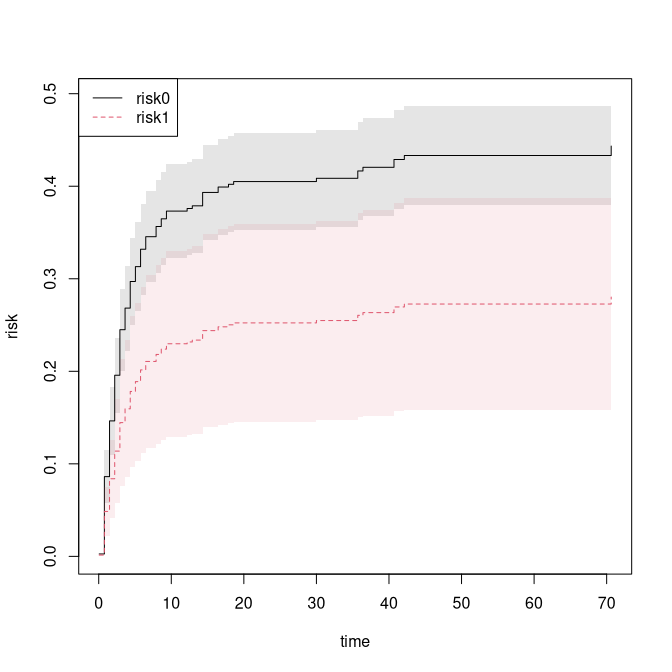
Now looking at the survival probability
ss <- phreg(Surv(time,event)~tcell+platelet+age,bmt)
sss <- survivalG(ss,bmt,time=50)
summary(sss)
#> G-estimator :
#>       Estimate Std.Err   2.5%  97.5%    P-value
#> risk0   0.6539 0.02709 0.6008 0.7070 9.218e-129
#> risk1   0.5640 0.05971 0.4470 0.6811  3.531e-21
#>
#> Average Treatment effect: difference (G-estimator) :
#>     Estimate Std.Err    2.5%   97.5% P-value
#> ps0 -0.08992  0.0629 -0.2132 0.03337  0.1529
#>
#> Average Treatment effect: ratio (G-estimator) :
#> log-ratio:
#>       Estimate   Std.Err       2.5%      97.5%   P-value
#> ps0 -0.1479231 0.1095247 -0.3625876 0.06674132 0.1768263
#> ratio:
#>  Estimate      2.5%     97.5%
#> 0.8624974 0.6958733 1.0690189
#>
#> Average Treatment effect:  survival-difference (G-estimator) :
#>       Estimate    Std.Err        2.5%     97.5%   P-value
#> ps0 0.08991862 0.06290398 -0.03337092 0.2132082 0.1528725
#>
#> Average Treatment effect: 1-G (survival)-ratio (G-estimator) :
#> log-ratio:
#>      Estimate   Std.Err       2.5%     97.5%   P-value
#> ps0 0.2309818 0.1503867 -0.0637708 0.5257343 0.1245583
#> ratio:
#> Estimate     2.5%    97.5%
#> 1.259836 0.938220 1.691701

Gtime <- survivalGtime(ss,bmt)
plot(Gtime)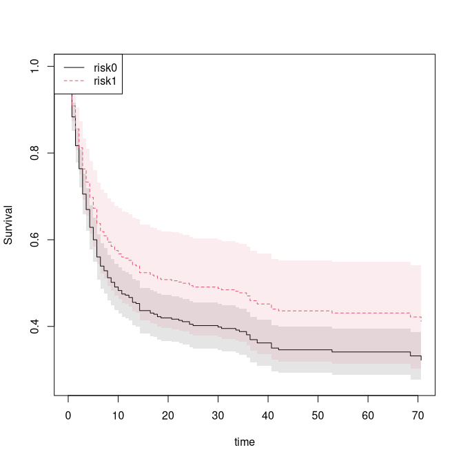
G-computation for the binomial regression
We compare with similar estimates using doubly robust estimating
equations via binregATE. The G-computation standardisation
can also be computed using a specialised function that uses less memory
and is faster for large data: binregG.
## survival situation
sr1 <- binregATE(Event(time,event)~tcell+platelet+age,bmt,cause=1,
         time=40, treat.model=tcell~platelet+age)
summary(sr1)
#>    n events
#>  408    241
#>
#>  408 clusters
#> coeffients:
#>              Estimate   Std.Err      2.5%     97.5% P-value
#> (Intercept)  0.676409  0.137007  0.407880  0.944939  0.0000
#> tcell1      -0.023675  0.346994 -0.703770  0.656420  0.9456
#> platelet    -0.492952  0.246158 -0.975412 -0.010492  0.0452
#> age          0.343939  0.115561  0.117444  0.570434  0.0029
#>
#> exp(coeffients):
#>             Estimate    2.5%  97.5%
#> (Intercept)  1.96680 1.50363 2.5727
#> tcell1       0.97660 0.49472 1.9279
#> platelet     0.61082 0.37704 0.9896
#> age          1.41049 1.12462 1.7690
#>
#> Average Treatment effects (G-formula) :
#>             Estimate    Std.Err       2.5%      97.5% P-value
#> treat0     0.6230976  0.0273827  0.5694284  0.6767667  0.0000
#> treat1     0.6177595  0.0731712  0.4743466  0.7611723  0.0000
#> treat:1-0 -0.0053381  0.0783973 -0.1589940  0.1483179  0.9457
#>
#> Average Treatment effects (double robust) :
#>            Estimate   Std.Err      2.5%     97.5% P-value
#> treat0     0.622698  0.027460  0.568878  0.676518   0.000
#> treat1     0.637785  0.085242  0.470714  0.804857   0.000
#> treat:1-0  0.015087  0.089442 -0.160215  0.190389   0.866

## relative risk effect
estimate(coef=sr1$riskDR,vcov=sr1$var.riskDR,f=function(p) p[2]/p[1],null=1)
#>        Estimate Std.Err   2.5% 97.5% P-value
#> treat1    1.024   0.144 0.7421 1.306  0.8664
#> ────────────────────────────────────────────────────────────
#> Null Hypothesis:
#>   [treat1] = 1
#>
#> chisq = 0.0283, df = 1, p-value = 0.8664

## competing risks
br1 <- binregATE(Event(time,cause)~tcell+platelet+age,bmt,cause=1,
         time=40,treat.model=tcell~platelet+age)
summary(br1)
#>    n events
#>  408    157
#>
#>  408 clusters
#> coeffients:
#>              Estimate   Std.Err      2.5%     97.5% P-value
#> (Intercept) -0.191519  0.130883 -0.448044  0.065007  0.1434
#> tcell1      -0.712880  0.351489 -1.401786 -0.023974  0.0425
#> platelet    -0.531919  0.244495 -1.011119 -0.052718  0.0296
#> age          0.432939  0.107314  0.222607  0.643271  0.0001
#>
#> exp(coeffients):
#>             Estimate    2.5%  97.5%
#> (Intercept)  0.82570 0.63888 1.0672
#> tcell1       0.49023 0.24616 0.9763
#> platelet     0.58748 0.36381 0.9486
#> age          1.54178 1.24933 1.9027
#>
#> Average Treatment effects (G-formula) :
#>            Estimate   Std.Err      2.5%     97.5% P-value
#> treat0     0.417746  0.027030  0.364768  0.470724  0.0000
#> treat1     0.267097  0.061849  0.145874  0.388319  0.0000
#> treat:1-0 -0.150649  0.067578 -0.283100 -0.018199  0.0258
#>
#> Average Treatment effects (double robust) :
#>            Estimate   Std.Err      2.5%     97.5% P-value
#> treat0     0.417121  0.027112  0.363983  0.470259  0.0000
#> treat1     0.227776  0.061240  0.107748  0.347803  0.0002
#> treat:1-0 -0.189345  0.066600 -0.319878 -0.058812  0.0045
and using the specialized function
br1 <- binreg(Event(time,cause)~tcell+platelet+age,bmt,cause=1,time=40)
Gbr1 <- binregG(br1,bmt,Avalues=NULL)
summary(Gbr1)
#> G-estimator :
#>       Estimate Std.Err   2.5%  97.5%   P-value
#> risk0   0.4177 0.02703 0.3648 0.4707 6.988e-54
#> risk1   0.2671 0.06185 0.1459 0.3883 1.571e-05
#>
#> Average Treatment effect: difference (G-estimator) :
#>    Estimate Std.Err    2.5%   97.5% P-value
#> pa  -0.1506 0.06758 -0.2831 -0.0182  0.0258
#>
#> Average Treatment effect: ratio (G-estimator) :
#> log-ratio:
#>      Estimate   Std.Err       2.5%      97.5%    P-value
#> pa -0.4472628 0.2406332 -0.9188953 0.02436964 0.06307095
#> ratio:
#>  Estimate      2.5%     97.5%
#> 0.6393758 0.3989595 1.0246690

## contrasting average age to 1+2-sd age, Avalues
Gbr2 <- binregG(br1,bmt,varname="age",Avalues=c(0,1,2))
summary(Gbr2)
#> G-estimator :
#>       Estimate Std.Err   2.5%  97.5%   P-value
#> risk0   0.3932 0.02537 0.3434 0.4429 3.738e-54
#> risk1   0.4964 0.03655 0.4248 0.5681 5.044e-42
#> risk2   0.5997 0.05531 0.4913 0.7081 2.136e-27
#>
#> Average Treatment effect: difference (G-estimator) :
#>      Estimate Std.Err    2.5%  97.5%   P-value
#> pa     0.1033 0.02605 0.05222 0.1543 7.345e-05
#> pa.1   0.2066 0.04996 0.10863 0.3045 3.564e-05
#>
#> Average Treatment effect: ratio (G-estimator) :
#> log-ratio:
#>     Estimate    Std.Err      2.5%     97.5%      P-value
#> pa 0.2332376 0.05402806 0.1273445 0.3391307 1.581845e-05
#> pa 0.4222406 0.08691473 0.2518908 0.5925903 1.185167e-06
#> ratio:
#>    Estimate     2.5%    97.5%
#> pa 1.262681 1.135808 1.403727
#> pa 1.525375 1.286456 1.808667
SessionInfo
sessionInfo()
#> R version 4.6.0 (2026-04-24)
#> Platform: x86_64-pc-linux-gnu
#> Running under: Ubuntu 24.04.4 LTS
#>
#> Matrix products: default
#> BLAS:   /home/kkzh/.asdf/installs/r/4.6.0/lib/R/lib/libRblas.so
#> LAPACK: /usr/lib/x86_64-linux-gnu/lapack/liblapack.so.3.12.0  LAPACK version 3.12.0
#>
#> locale:
#>  [1] LC_CTYPE=en_US.UTF-8       LC_NUMERIC=C
#>  [3] LC_TIME=en_US.UTF-8        LC_COLLATE=en_US.UTF-8
#>  [5] LC_MONETARY=en_US.UTF-8    LC_MESSAGES=en_US.UTF-8
#>  [7] LC_PAPER=en_US.UTF-8       LC_NAME=C
#>  [9] LC_ADDRESS=C               LC_TELEPHONE=C
#> [11] LC_MEASUREMENT=en_US.UTF-8 LC_IDENTIFICATION=C
#>
#> time zone: Europe/Copenhagen
#> tzcode source: system (glibc)
#>
#> attached base packages:
#> [1] splines   stats     graphics  grDevices utils     datasets  methods
#> [8] base
#>
#> other attached packages:
#> [1] timereg_2.0.7  survival_3.8-6 mets_1.3.10
#>
#> loaded via a namespace (and not attached):
#>  [1] vctrs_0.7.3            cli_3.6.6              knitr_1.51
#>  [4] rlang_1.2.0            xfun_0.57              KernSmooth_2.23-26
#>  [7] otel_0.2.0             glue_1.8.1             future.apply_1.20.2
#> [10] listenv_0.10.1         lava_1.9.1             stats4_4.6.0
#> [13] grid_4.6.0             evaluate_1.0.5         lifecycle_1.0.5
#> [16] yaml_2.3.12            mvtnorm_1.3-7          numDeriv_2016.8-1.1
#> [19] compiler_4.6.0         codetools_0.2-20       Rcpp_1.1.1-1.1
#> [22] ucminf_1.2.3           future_1.70.0          lattice_0.22-9
#> [25] digest_0.6.39          pillar_1.11.1          parallelly_1.47.0
#> [28] parallel_4.6.0         Matrix_1.7-5           tools_4.6.0
#> [31] RcppArmadillo_15.2.6-1 globals_0.19.1