-
Multivariate Event Times (
mets)
- Installation
- Citation
- Examples: Twins Polygenic modelling
- Examples: Twins Polygenic modelling time-to-events Data
- Examples: Twins Concordance for time-to-events Data
- Examples: Cox model, RMST
- Examples: Cox model IPTW
- Examples: Competing risks regression, Binomial Regression
- Examples: Competing risks regression, Fine-Gray/Logistic link
- Examples: Marginal mean for recurrent events
- Examples: Ghosh-Lin for recurrent events
- Examples: Fixed time modelling for recurrent events
- Examples: Cumulative Medical Cost
- Examples: Regression for RMST/Restricted mean survival for survival and competing risks using IPCW
- Examples: Average treatment effects (ATE) for survival or competing risks
- Examples: While Alive estimands for recurrent events
Implementation of various statistical models for multivariate event history data doi:10.1007/s10985-013-9244-x. Including multivariate cumulative incidence models doi:10.1002/sim.6016, and bivariate random effects probit models (Liability models) doi:10.1016/j.csda.2015.01.014. Modern methods for survival analysis, including regression modelling (Cox, Fine-Gray, Ghosh-Lin, Binomial regression) with fast computation of influence functions. Restricted mean survival time regression and years lost for competing risks. Average treatment effects and G-computation. All functions can be used with clusters and will work for large data.
Installation
install.packages("mets")The development version may be installed directly from github (requires Rtools on windows and development tools (+Xcode) for Mac OS X):
remotes::install_github("kkholst/mets", dependencies="Suggests")or to get development version
remotes::install_github("kkholst/mets",ref="develop")Citation
To cite the mets package please use one of the following references
Thomas H. Scheike and Klaus K. Holst (2022). A Practical Guide to Family Studies with Lifetime Data. Annual Review of Statistics and Its Application 9, pp. 47-69. doi: http://dx.doi.org/10.1146/annurev-statistics-040120-024253
Thomas H. Scheike and Klaus K. Holst and Jacob B. Hjelmborg (2013). Estimating heritability for cause specific mortality based on twin studies. Lifetime Data Analysis. http://dx.doi.org/10.1007/s10985-013-9244-x
Klaus K. Holst and Thomas H. Scheike Jacob B. Hjelmborg (2015). The Liability Threshold Model for Censored Twin Data. Computational Statistics and Data Analysis. http://dx.doi.org/10.1016/j.csda.2015.01.014
BibTeX:
@Article{,
  title = {A Practical Guide to Family Studies with Lifetime Data},
  author = {Thomas H. Scheike and Klaus K. Holst},
  year = {2014},
  volume = {9},
  pages = {47-69},
  journal = {Annual Review of Statistics and Its Application},
  doi = {10.1146/annurev-statistics-040120-024253},
}

@Article{,
  title={Estimating heritability for cause specific mortality based on twin studies},
  author={Scheike, Thomas H. and Holst, Klaus K. and Hjelmborg, Jacob B.},
  year={2013},
  issn={1380-7870},
  journal={Lifetime Data Analysis},
  doi={10.1007/s10985-013-9244-x},
  url={http://dx.doi.org/10.1007/s10985-013-9244-x},
  publisher={Springer US},
  keywords={Cause specific hazards; Competing risks; Delayed entry;
        Left truncation; Heritability; Survival analysis},
  pages={1-24},
  language={English}
}

@Article{,
  title={The Liability Threshold Model for Censored Twin Data},
  author={Holst, Klaus K. and Scheike, Thomas H. and Hjelmborg, Jacob B.},
  year={2015},
  doi={10.1016/j.csda.2015.01.014},
  url={http://dx.doi.org/10.1016/j.csda.2015.01.014},
  journal={Computational Statistics and Data Analysis}
}
Examples: Twins Polygenic modelling
First considering standard twin modelling (ACE, AE, ADE, and more models)
# simulated data with pairs of observations in twins on long #data format
set.seed(1)
d <- twinsim(1000, b1=c(1,-1), b2=c(), acde=c(1,1,0,1))
# Polygenic model with Additive genetic effects, and shared and individual environmental effects (ACE)
ace <- twinlm(y ~ 1, data=d, DZ="DZ", zyg="zyg", id="id")
ace
#>        Estimate Std. Error Z value  Pr(>|z|)
#> y     -0.019439   0.041817 -0.4649     0.642
#> sd(A)  0.902004   0.203739  4.4273 9.544e-06
#> sd(C)  1.137025   0.132852  8.5586 < 2.2e-16
#> sd(E)  1.728992   0.037408 46.2194 < 2.2e-16
#>
#> MZ-pairs DZ-pairs
#>     1000     1000
#>
#> Variance decomposition:
#>   Estimate 2.5%    97.5%
#> A 0.15966  0.01867 0.30065
#> C 0.25370  0.13920 0.36820
#> E 0.58664  0.53677 0.63650
#>
#>
#>                          Estimate 2.5%    97.5%
#> Broad-sense heritability 0.15966  0.01867 0.30065
#>
#>                        Estimate 2.5%    97.5%
#> Correlation within MZ: 0.41336  0.36229 0.46196
#> Correlation within DZ: 0.33353  0.27933 0.38561
#>
#> 'log Lik.' -8779.953 (df=4)
#> AIC: 17567.91
#> BIC: 17590.31
# An AE-model could be fitted as
ae <- twinlm(y ~ 1, data=d, DZ="DZ", zyg="zyg", id="id", type="ae")
# AIC
AIC(ae)-AIC(ace)
#> [1] 15.20656
# To adjust for the covariates we simply alter the formula statement
ace2 <- twinlm(y ~ x1+x2, data=d, DZ="DZ", zyg="zyg", id="id", type="ace")
 ## Summary/GOF
summary(ace2)
#>        Estimate Std. Error  Z value Pr(>|z|)
#> y     -0.026049   0.034844  -0.7476   0.4547
#> sd(A)  1.066060   0.072890  14.6256   <2e-16
#> sd(C)  0.980740   0.073569  13.3309   <2e-16
#> sd(E)  0.979980   0.021887  44.7736   <2e-16
#> y~x1   1.006963   0.021900  45.9807   <2e-16
#> y~x2  -0.993802   0.021962 -45.2512   <2e-16
#>
#> MZ-pairs DZ-pairs
#>     1000     1000
#>
#> Variance decomposition:
#>   Estimate 2.5%    97.5%
#> A 0.37156  0.27300 0.47012
#> C 0.31446  0.22643 0.40250
#> E 0.31398  0.28381 0.34414
#>
#>
#>                          Estimate 2.5%    97.5%
#> Broad-sense heritability 0.37156  0.27300 0.47012
#>
#>                        Estimate 2.5%    97.5%
#> Correlation within MZ: 0.68602  0.65467 0.71502
#> Correlation within DZ: 0.50024  0.45538 0.54257
#>
#> 'log Lik.' -7449.697 (df=6)
#> AIC: 14911.39
#> BIC: 14945
Examples: Twins Polygenic modelling time-to-events Data
In the context of time-to-events data we consider the “Liability Threshold model” with IPCW adjustment for censoring.
First we fit the bivariate probit model (same marginals in MZ and DZ twins but different correlation parameter). Here we evaluate the risk of getting cancer before the last double cancer event (95 years)
data(prt)
prt0 <-  force.same.cens(prt, cause="status", cens.code=0, time="time", id="id")
prt0$country <- relevel(prt0$country, ref="Sweden")
prt_wide <- fast.reshape(prt0, id="id", num="num", varying=c("time","status","cancer"))
prt_time <- subset(prt_wide,  cancer1 & cancer2, select=c(time1, time2, zyg))
tau <- 95
tt <- seq(70, tau, length.out=5) ## Time points to evaluate model in

b0 <- bptwin.time(cancer ~ 1, data=prt0, id="id", zyg="zyg", DZ="DZ", type="cor",
              cens.formula=Surv(time,status==0)~zyg, breaks=tau)
summary(b0)
#>
#>                Estimate   Std.Err        Z   p-value
#> (Intercept)   -1.348188  0.026276 -51.3086 < 2.2e-16 ***
#> atanh(rho) MZ  0.735992  0.087838   8.3789 < 2.2e-16 ***
#> atanh(rho) DZ  0.353023  0.068234   5.1737 2.295e-07 ***
#> ---
#> Signif. codes:  0 '***' 0.001 '**' 0.01 '*' 0.05 '.' 0.1 ' ' 1
#>
#>  Total MZ/DZ Complete pairs MZ/DZ
#>  1994/3618   997/1809
#>
#>                            Estimate 2.5%    97.5%
#> Tetrachoric correlation MZ 0.62672  0.51081 0.72024
#> Tetrachoric correlation DZ 0.33905  0.21584 0.45164
#>
#> MZ:
#>                      Estimate 2.5%    97.5%
#> Concordance          0.03504  0.02779 0.04409
#> Casewise Concordance 0.39458  0.31876 0.47584
#> Marginal             0.08880  0.08086 0.09743
#> Rel.Recur.Risk       4.44351  3.50521 5.38182
#> log(OR)              2.34131  1.87105 2.81157
#> DZ:
#>                      Estimate 2.5%    97.5%
#> Concordance          0.01952  0.01449 0.02625
#> Casewise Concordance 0.21983  0.16667 0.28415
#> Marginal             0.08880  0.08086 0.09743
#> Rel.Recur.Risk       2.47556  1.81096 3.14016
#> log(OR)              1.23088  0.81020 1.65156
#>
#>                          Estimate 2.5%    97.5%
#> Broad-sense heritability 0.57533  0.25790 0.89276
#>
#>
#> Event of interest before time 95
Liability threshold model with ACE random effects structure
b1 <- bptwin.time(cancer ~ 1, data=prt0, id="id", zyg="zyg", DZ="DZ", type="ace",
           cens.formula=Surv(time,status==0)~zyg, breaks=tau)
summary(b1)
#>
#>             Estimate  Std.Err        Z p-value
#> (Intercept) -2.20664  0.16463 -13.4034  <2e-16 ***
#> log(var(A))  0.43260  0.39149   1.1050  0.2691
#> log(var(C)) -1.98289  2.52342  -0.7858  0.4320
#> ---
#> Signif. codes:  0 '***' 0.001 '**' 0.01 '*' 0.05 '.' 0.1 ' ' 1
#>
#>  Total MZ/DZ Complete pairs MZ/DZ
#>  1994/3618   997/1809
#>
#>                    Estimate 2.5%     97.5%
#> A                   0.57533  0.25790  0.89276
#> C                   0.05139 -0.20836  0.31114
#> E                   0.37328  0.26874  0.47782
#> MZ Tetrachoric Cor  0.62672  0.51081  0.72024
#> DZ Tetrachoric Cor  0.33905  0.21584  0.45164
#>
#> MZ:
#>                      Estimate 2.5%    97.5%
#> Concordance          0.03504  0.02779 0.04409
#> Casewise Concordance 0.39458  0.31876 0.47584
#> Marginal             0.08880  0.08086 0.09743
#> Rel.Recur.Risk       4.44351  3.50520 5.38182
#> log(OR)              2.34131  1.87104 2.81157
#> DZ:
#>                      Estimate 2.5%    97.5%
#> Concordance          0.01952  0.01449 0.02625
#> Casewise Concordance 0.21983  0.16667 0.28415
#> Marginal             0.08880  0.08086 0.09743
#> Rel.Recur.Risk       2.47556  1.81096 3.14016
#> log(OR)              1.23088  0.81020 1.65156
#>
#>                          Estimate 2.5%    97.5%
#> Broad-sense heritability 0.57533  0.25790 0.89276
#>
#>
#> Event of interest before time 95
Examples: Twins Concordance for time-to-events Data
data(prt) ## Prostate data example (sim)

## Bivariate competing risk, concordance estimates
p33 <- bicomprisk(Event(time,status)~strata(zyg)+id(id),
                  data=prt, cause=c(2,2), return.data=1, prodlim=TRUE)
#> Strata 'DZ'
#> Strata 'MZ'

p33dz <- p33$model$"DZ"$comp.risk
p33mz <- p33$model$"MZ"$comp.risk

## Probability weights based on Aalen's additive model (same censoring within pair)
prtw <- ipw(Surv(time,status==0)~country+zyg, data=prt,
            obs.only=TRUE, same.cens=TRUE,
            cluster="id", weight.name="w")

## Marginal model (wrongly ignoring censorings)
bpmz <- biprobit(cancer~1 + cluster(id),
                 data=subset(prt,zyg=="MZ"), eqmarg=TRUE)

## Extended liability model
bpmzIPW <- biprobit(cancer~1 + cluster(id),
                    data=subset(prtw,zyg=="MZ"),
                    weights="w")
smz <- summary(bpmzIPW)

## Concordance
plot(p33mz,ylim=c(0,0.1),axes=FALSE, automar=FALSE,atrisk=FALSE,background=TRUE,background.fg="white")
axis(2); axis(1)

abline(h=smz$prob["Concordance",],lwd=c(2,1,1),col="darkblue")
## Wrong estimates:
abline(h=summary(bpmz)$prob["Concordance",],lwd=c(2,1,1),col="lightgray",lty=2)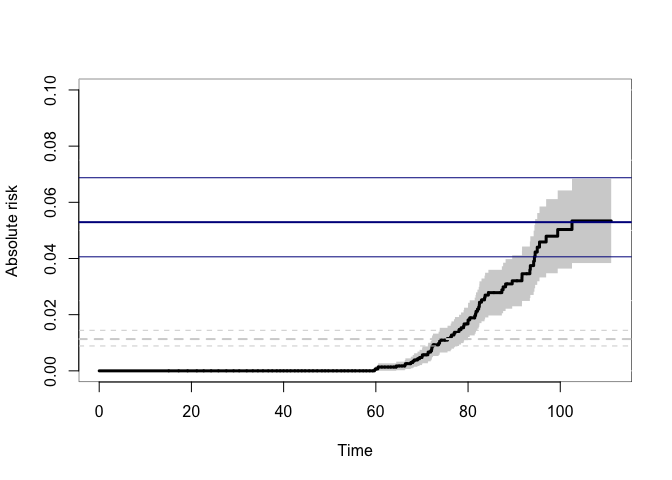
Examples: Cox model, RMST
We can fit the Cox model and compute many useful summaries, such as restricted mean survival and standardized treatment effects (G-estimation). First estimating the standardized survival
 data(bmt)
 bmt$time <- bmt$time+runif(408)*0.001
 bmt$event <- (bmt$cause!=0)*1
 dfactor(bmt) <- tcell.f~tcell

 ss <- phreg(Surv(time,event)~tcell.f+platelet+age,bmt)
 summary(survivalG(ss,bmt,50))
#> G-estimator :
#>       Estimate Std.Err   2.5%  97.5%    P-value
#> risk0   0.6539 0.02708 0.6008 0.7070 9.119e-129
#> risk1   0.5641 0.05973 0.4470 0.6811  3.600e-21
#>
#> Average Treatment effect: difference (G-estimator) :
#>     Estimate Std.Err    2.5%   97.5% P-value
#> ps0 -0.08982 0.06293 -0.2132 0.03352  0.1535
#>
#> Average Treatment effect: ratio (G-estimator) :
#> log-ratio:
#>         Estimate  Std.Err       2.5%      97.5%   P-value
#> [ps0] -0.1477619 0.109562 -0.3624994 0.06697567 0.1774462
#> ratio:
#>  Estimate      2.5%     97.5%
#> 0.8626365 0.6959347 1.0692695
#>
#> Average Treatment effect:  survival-difference (G-estimator) :
#>       Estimate    Std.Err        2.5%     97.5%   P-value
#> ps0 0.08981829 0.06292811 -0.03351854 0.2131551 0.1534889
#>
#> Average Treatment effect: 1-G (survival)-ratio (G-estimator) :
#> log-ratio:
#>       Estimate   Std.Err        2.5%     97.5%   P-value
#> [ps0] 0.230711 0.1504459 -0.06415759 0.5255796 0.1251491
#> ratio:
#>  Estimate      2.5%     97.5%
#> 1.2594952 0.9378572 1.6914390

 sst <- survivalGtime(ss,bmt,n=50)
 plot(sst,type=c("survival","risk","survival.ratio")[1])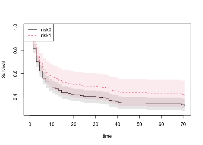
Based on the phreg we can also compute the restricted mean survival time and years lost (via Kaplan-Meier estimates). The function does it for all times at once and can be plotted as restricted mean survival or years lost at the different time horizons
 out1 <- phreg(Surv(time,cause!=0)~strata(tcell,platelet),data=bmt)

 rm1 <- resmean_phreg(out1, times=c(50))
 summary(rm1)
#>                     strata times    rmean se.rmean    lower    upper years.lost
#> tcell=0, platelet=0      0    50 20.48245 1.411055 17.89542 23.44348   29.51755
#> tcell=0, platelet=1      1    50 28.33071 2.196175 24.33733 32.97934   21.66929
#> tcell=1, platelet=0      2    50 22.74596 4.053717 16.04005 32.25544   27.25404
#> tcell=1, platelet=1      3    50 26.11565 4.230688 19.01112 35.87517   23.88435
 par(mfrow=c(1, 2))
 plot(rm1,se=1)
 plot(rm1,years.lost=TRUE,se=1)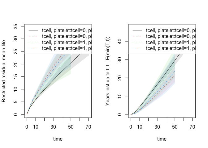
For competing risks the years lost can be decomposed into different causes and is based on the integrated Aalen-Johansen estimators for the different strata
 ## years.lost decomposed into causes
drm1 <- cif_yearslost(Event(time,cause)~strata(tcell,platelet),data=bmt,times=50)
 par(mfrow=c(1,2)); plot(drm1,cause=1,se=1); title(main="Cause 1"); plot(drm1,cause=2,se=1); title(main="Cause 2")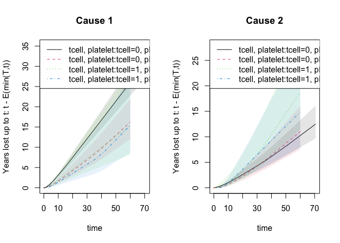
 summary(drm1)
#> $estimate
#>                     strata times   intF_1    intF_2 se.intF_1 se.intF_2
#> tcell=0, platelet=0      0    50 21.36784  8.149711  1.476647  1.094520
#> tcell=0, platelet=1      1    50 12.97924  8.690047  2.047516  1.712441
#> tcell=1, platelet=0      2    50 12.64543 14.608610  4.089981  3.730259
#> tcell=1, platelet=1      3    50 11.80934 12.075008  3.673701  3.890207
#>                     total.years.lost lower_intF_1 upper_intF_1 lower_intF_2
#> tcell=0, platelet=0         29.51755    18.661106     24.46717     6.263606
#> tcell=0, platelet=1         21.66929     9.527297     17.68191     5.905902
#> tcell=1, platelet=0         27.25404     6.708487     23.83649     8.856404
#> tcell=1, platelet=1         23.88435     6.418453     21.72807     6.421784
#>                     upper_intF_2
#> tcell=0, platelet=0     10.60376
#> tcell=0, platelet=1     12.78669
#> tcell=1, platelet=0     24.09685
#> tcell=1, platelet=1     22.70487
Computations are again done for all time horizons at once as illustrated in the plot.
Examples: Cox model IPTW
We can fit the Cox model with inverse probability of treatment weights based on logistic regression. The treatment weights can be time-dependent and then multiplicative weights are applied (see details and vignette).
data(bmt)
bmt$time <- bmt$time+runif(408)*0.001
bmt$id <- seq_len(nrow(bmt))
bmt$event <- (bmt$cause!=0)*1
dfactor(bmt) <- tcell.f~tcell

fit <- phreg_IPTW(Surv(time,event)~tcell.f+cluster(id),data=bmt,treat.model=tcell.f~platelet+age)
summary(fit)
#>
#>    n events
#>  408    248
#>
#>  408 clusters
#> coeffients:
#>           Estimate      S.E.   dU^-1/2 P-value
#> tcell.f1 -0.108497  0.199556  0.089653  0.5867
#>
#> exp(coeffients):
#>          Estimate    2.5%  97.5%
#> tcell.f1  0.89718 0.60676 1.3266
head(IC(fit))
#>    tcell.f1
#> 1 -1.639241
#> 2 -1.669074
#> 3 -1.749761
#> 4 -1.745988
#> 5 -1.625416
#> 6 -1.793372
Examples: Competing risks regression, Binomial Regression
We can fit the logistic regression model at a specific time-point with IPCW adjustment
data(bmt); bmt$time <- bmt$time+runif(408)*0.001
# logistic regression with IPCW binomial regression
out <- binreg(Event(time,cause)~tcell+platelet,bmt,time=50)
summary(out)
#>    n events
#>  408    160
#>
#>  408 clusters
#> coeffients:
#>              Estimate   Std.Err      2.5%     97.5% P-value
#> (Intercept) -0.180371  0.126757 -0.428811  0.068068  0.1547
#> tcell       -0.418682  0.345438 -1.095729  0.258364  0.2255
#> platelet    -0.436959  0.240977 -0.909266  0.035349  0.0698
#>
#> exp(coeffients):
#>             Estimate    2.5%  97.5%
#> (Intercept)  0.83496 0.65128 1.0704
#> tcell        0.65791 0.33430 1.2948
#> platelet     0.64600 0.40282 1.0360
head(IC(out))
#>           [,1]     [,2]    [,3]
#> [1,] -2.834084 1.633524 2.52025
#> [2,] -2.834084 1.633524 2.52025
#> [3,] -2.834084 1.633524 2.52025
#> [4,] -2.834084 1.633524 2.52025
#> [5,] -2.834084 1.633524 2.52025
#> [6,] -2.834084 1.633524 2.52025
 predict(out,data.frame(tcell=c(0,1),platelet=c(1,1)),se=TRUE)
#>        pred         se     lower     upper
#> 1 0.3503890 0.04848653 0.2553554 0.4454226
#> 2 0.2619201 0.06969710 0.1253138 0.3985265
Examples: Competing risks regression, Fine-Gray/Logistic link
We can fit the Fine-Gray model and the logit-link competing risks model (using IPCW adjustment). Starting with the logit-link model
data(bmt)
bmt$time <- bmt$time+runif(nrow(bmt))*0.01
bmt$id <- 1:nrow(bmt)
## logistic link  OR interpretation
 or=cifreg(Event(time,cause)~strata(tcell)+platelet+age,data=bmt,cause=1)
summary(or)
#>
#>    n events
#>  408    161
#>
#>  408 clusters
#> coeffients:
#>           Estimate      S.E.   dU^-1/2 P-value
#> platelet -0.454572  0.235415  0.187997  0.0535
#> age       0.390181  0.097675  0.083636  0.0001
#>
#> exp(coeffients):
#>          Estimate    2.5%  97.5%
#> platelet  0.63472 0.40013 1.0069
#> age       1.47725 1.21987 1.7889
par(mfrow=c(1,2))
 ## to see baseline
plot(or)

 # predictions
nd <- data.frame(tcell=c(1,0),platelet=0,age=0)
pll <- predict(or,nd)
plot(pll)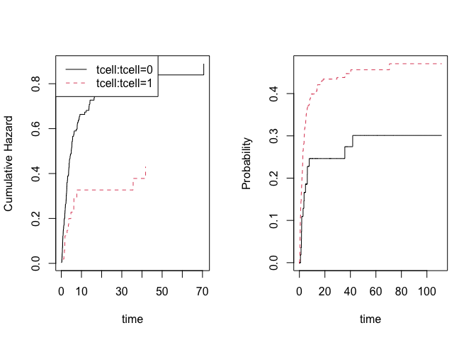
Similarly, the Fine-Gray model can be estimated using IPCW adjustment
 ## Fine-Gray model
 fg=cifreg(Event(time,cause)~strata(tcell)+platelet+age,data=bmt,cause=1,propodds=NULL)
 summary(fg)
#>
#>    n events
#>  408    161
#>
#>  408 clusters
#> coeffients:
#>           Estimate      S.E.   dU^-1/2 P-value
#> platelet -0.424749  0.180772  0.187820  0.0188
#> age       0.341971  0.079862  0.086284  0.0000
#>
#> exp(coeffients):
#>          Estimate    2.5%  97.5%
#> platelet  0.65393 0.45884 0.9320
#> age       1.40772 1.20375 1.6462
## baselines
plot(fg)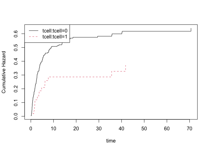
nd <- data.frame(tcell=c(1,0),platelet=0,age=0)
pfg <- predict(fg,nd,se=1)
plot(pfg,se=1)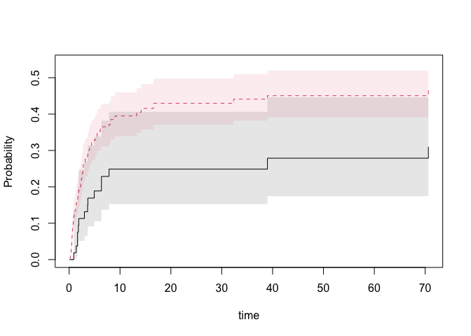
## influence functions of regression coefficients
head(iid(fg))
#>         platelet           age
#> [1,] 0.004953478  0.0001245648
#> [2,] 0.005348496 -0.0022341772
#> [3,] 0.006069271 -0.0087212019
#> [4,] 0.006043180 -0.0084186443
#> [5,] 0.004732097  0.0011839243
#> [6,] 0.006331457 -0.0121685409
and we can get standard errors for predictions based on the influence functions of the baseline and the regression coefficients (these are used in the predict function)
baseid <- iidBaseline(fg,time=40)
FGprediid(baseid,nd)
#>           pred     se-log     lower     upper
#> [1,] 0.2787465 0.23977109 0.1742272 0.4459672
#> [2,] 0.4506249 0.07265694 0.3908134 0.5195901
further G-estimation can be done
 dfactor(bmt) <- tcell.f~tcell
 fg1 <- cifreg(Event(time,cause)~tcell.f+platelet+age,bmt,cause=1,propodds=NULL)
 summary(survivalG(fg1,bmt,50))
#> G-estimator :
#>       Estimate Std.Err   2.5%  97.5%   P-value
#> risk0   0.4332 0.02749 0.3793 0.4871 6.331e-56
#> risk1   0.2726 0.05861 0.1577 0.3875 3.301e-06
#>
#> Average Treatment effect: difference (G-estimator) :
#>     Estimate Std.Err   2.5%    97.5% P-value
#> ps0  -0.1606 0.06351 -0.285 -0.03609 0.01146
#>
#> Average Treatment effect: ratio (G-estimator) :
#> log-ratio:
#>        Estimate   Std.Err       2.5%       97.5%    P-value
#> [ps0] -0.463091 0.2211651 -0.8965667 -0.02961528 0.03627159
#> ratio:
#>  Estimate      2.5%     97.5%
#> 0.6293354 0.4079679 0.9708190
Examples: Marginal mean for recurrent events
We can estimate the expected number of events non-parametrically and get standard errors for this estimator
data(hfactioncpx12)
dtable(hfactioncpx12,~status)
#>
#> status
#>    0    1    2
#>  617 1391  124

gl1 <- recurrent_marginal(Event(entry,time,status)~strata(treatment)+cluster(id),hfactioncpx12,cause=1,death.code=2)
summary(gl1,times=1:5)
#> [[1]]
#>       new.time      mean         se   CI-2.5% CI-97.5% strata
#> 325          1 0.8737156 0.06783343 0.7503858 1.017315      0
#> 555          2 1.5718563 0.09572955 1.3949953 1.771140      0
#> 682          3 2.1184963 0.11385721 1.9066915 2.353829      0
#> 748          4 2.6815219 0.15451005 2.3951619 3.002118      0
#> 748.1        5 2.6815219 0.15451005 2.3951619 3.002118      0
#>
#> [[2]]
#>       new.time      mean         se   CI-2.5%  CI-97.5% strata
#> 284          1 0.7815557 0.06908585 0.6572305 0.9293989      1
#> 499          2 1.4534055 0.10315606 1.2646561 1.6703258      1
#> 601          3 1.9240624 0.12165771 1.6998008 2.1779119      1
#> 645          4 2.3134997 0.14963892 2.0380418 2.6261880      1
#> 645.1        5 2.3134997 0.14963892 2.0380418 2.6261880      1
plot(gl1,se=1)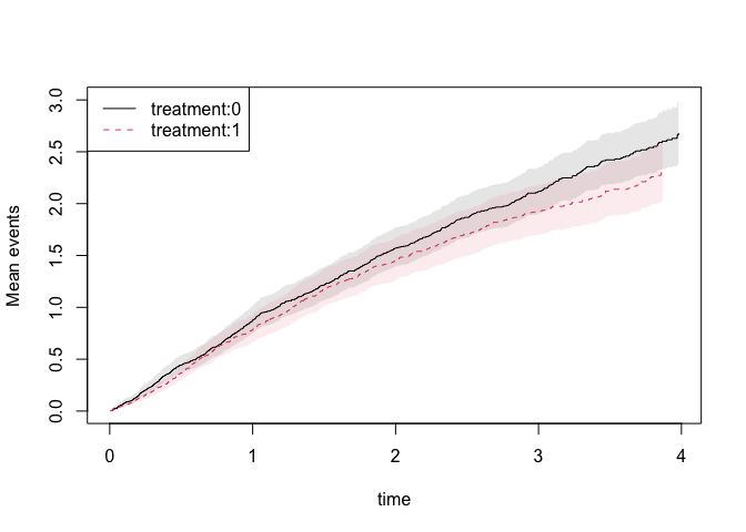
Examples: Ghosh-Lin for recurrent events
We can fit the Ghosh-Lin model for the expected number of events observed before dying (using IPCW adjustment and get predictions)
data(hfactioncpx12)
dtable(hfactioncpx12,~status)
#>
#> status
#>    0    1    2
#>  617 1391  124

gl1 <- recreg(Event(entry,time,status)~treatment+cluster(id),hfactioncpx12,cause=1,death.code=2)
summary(gl1)
#>
#>     n events
#>  2132   1391
#>
#>  741 clusters
#> coeffients:
#>             Estimate      S.E.   dU^-1/2 P-value
#> treatment1 -0.110404  0.078656  0.053776  0.1604
#>
#> exp(coeffients):
#>            Estimate    2.5%  97.5%
#> treatment1  0.89547 0.76754 1.0447

## influence functions of regression coefficients
head(iid(gl1))
#>      treatment1
#> 1 -1.266428e-04
#> 2 -6.112340e-04
#> 3  2.885192e-03
#> 4  1.308207e-03
#> 5  5.404664e-05
#> 6  2.229380e-03
and we can get standard errors for predictions based on the influence functions of the baseline and the regression coefficients
 nd=data.frame(treatment=levels(hfactioncpx12$treatment),id=1)
 pfg <- predict(gl1,nd,se=1)
 summary(pfg,times=1:5)
#> $pred
#>              Lamt     Lamt     Lamt     Lamt     Lamt
#> strata0 0.8573256 1.592252 2.121181 2.635437 2.635437
#> strata0 0.7677110 1.425817 1.899458 2.359959 2.359959
#>
#> $se.pred
#>       seLamt     seLamt    seLamt    seLamt    seLamt
#> 1 0.05719895 0.08818784 0.1096157 0.1429941 0.1429941
#> 2 0.05763288 0.09495475 0.1184567 0.1484200 0.1484200
#>
#> $lower
#>              [,1]     [,2]     [,3]     [,4]     [,5]
#> strata0 0.7522383 1.428458 1.916860 2.369561 2.369561
#> strata0 0.6626698 1.251343 1.680916 2.086276 2.086276
#>
#> $upper
#>              [,1]     [,2]     [,3]     [,4]     [,5]
#> strata0 0.9770936 1.774827 2.347281 2.931145 2.931145
#> strata0 0.8894025 1.624617 2.146415 2.669546 2.669546
#>
#> $times
#> [1] 1 2 3 4 5
#>
#> attr(,"class")
#> [1] "summarypredictrecreg"
 plot(pfg,se=1)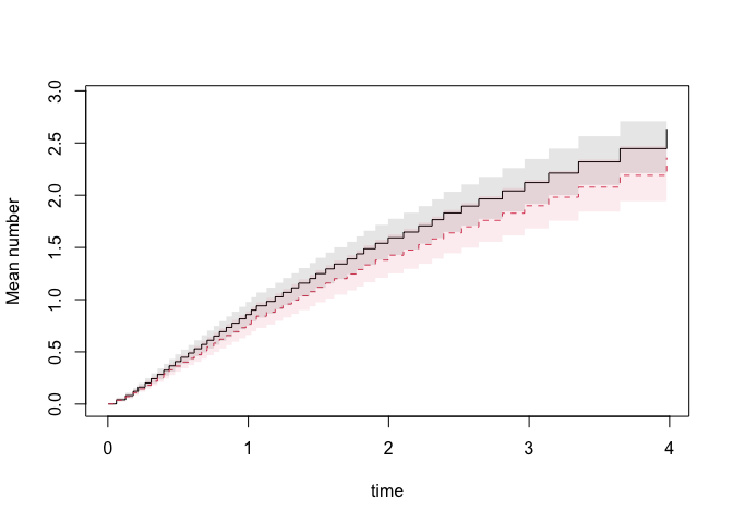
The influence functions of the baseline and regression coefficients at a specific time-point can be obtained
baseid <- iidBaseline(gl1,time=2)
dd <- data.frame(treatment=levels(hfactioncpx12$treatment),id=1)
GLprediid(baseid,dd)
#>          pred     se-log    lower    upper
#> [1,] 1.596065 0.05530215 1.432113 1.778786
#> [2,] 1.429231 0.06660096 1.254329 1.628521
and G-computation
 hfactioncpx12$age <- (50+rnorm(741)*4)[hfactioncpx12$id]

 GLout <- recreg(Event(entry,time,status)~treatment+age,data=hfactioncpx12,cause=1,death.code=2)
 summary(GLout)
#>
#>     n events
#>  2132   1391
#>
#>  2132 clusters
#> coeffients:
#>              Estimate       S.E.    dU^-1/2 P-value
#> treatment1 -0.1131085  0.0640898  0.0538154  0.0776
#> age         0.0086223  0.0079803  0.0066607  0.2799
#>
#> exp(coeffients):
#>            Estimate    2.5%  97.5%
#> treatment1  0.89305 0.78763 1.0126
#> age         1.00866 0.99301 1.0246
 summary(survivalG(GLout,hfactioncpx12,time=4))
#> G-estimator :
#>       Estimate Std.Err  2.5% 97.5%    P-value
#> risk0    2.640  0.1203 2.404 2.876 1.067e-106
#> risk1    2.358  0.1165 2.130 2.586  3.838e-91
#>
#> Average Treatment effect: difference (G-estimator) :
#>    Estimate Std.Err    2.5%   97.5% P-value
#> p1  -0.2824  0.1597 -0.5953 0.03059 0.07699
#>
#> Average Treatment effect: ratio (G-estimator) :
#> log-ratio:
#>        Estimate    Std.Err       2.5%      97.5%    P-value
#> [p1] -0.1131085 0.06408982 -0.2387222 0.01250527 0.07759015
#> ratio:
#>  Estimate      2.5%     97.5%
#> 0.8930538 0.7876336 1.0125838
Examples: Fixed time modelling for recurrent events
We can fit a log-link regression model at 2 years for the expected number of events observed before dying (using IPCW adjustment)
data(hfactioncpx12)

e2 <- recregIPCW(Event(entry,time,status)~treatment+cluster(id),hfactioncpx12,cause=1,death.code=2,time=2)
summary(e2)
#>    n events
#>  741   1052
#>
#>  741 clusters
#> coeffients:
#>              Estimate   Std.Err      2.5%     97.5% P-value
#> (Intercept)  0.452430  0.060814  0.333236  0.571624  0.0000
#> treatment1  -0.078322  0.093560 -0.261696  0.105052  0.4025
#>
#> exp(coeffients):
#>             Estimate    2.5%  97.5%
#> (Intercept)  1.57213 1.39548 1.7711
#> treatment1   0.92467 0.76974 1.1108
head(iid(e2))
#>            [,1]          [,2]
#> 1  1.959479e-04 -2.266440e-04
#> 2  2.237613e-03 -2.227140e-03
#> 3 -9.349773e-06  1.293789e-03
#> 4 -9.653029e-04  9.653029e-04
#> 5 -1.203962e-04  6.744236e-05
#> 6 -2.861359e-03  2.871831e-03
Examples: Cumulative Medical Cost
Estimate mean cumulative cost (see also vignette)
library(mets)
data(hfactioncpx12)
hf <- hfactioncpx12
hf$severity <- abs((5+rnorm(741)*2))[hf$id]

## marginal mean using formula
outNZ <- recurrent_marginal(Event(entry,time,status)~strata(treatment)+cluster(id)
             +marks(severity),hf,cause=1,death.code=2)
plot(outNZ,se=TRUE)
summary(outNZ,times=3)
For comparison we also compute the IPCW estimates at time 3, using the linear model, and note that they are identical. Standard errors are however based on different formula that are asymptotically equivalent, and we note that they are very similar.
{r} outNZ3 <- recregIPCW(Event(entry,time,status)~-1+treatment+cluster(id)+marks(severity),data=hf, cause=1,death.code=2,time=3,cens.model=~strata(treatment),model="lin") summary(outNZ3) head(iid(outNZ3))
We also apply the semiparametric proportional cost model with IPCW adjustment:
{r} propNZ <- recreg(Event(entry,time,status)~treatment+marks(severity)+cluster(id),data=hf,cause=1,death.code=2) summary(propNZ) plot(propNZ,main="Baselines")
Examples: Regression for RMST/Restricted mean survival for survival and competing risks using IPCW
RMST can be computed using the Kaplan-Meier (via phreg) and the for competing risks via the cumulative incidence functions, but we can also get these estimates via IPCW adjustment and then we can do regression
 ### same as Kaplan-Meier for full censoring model
 bmt$int <- with(bmt,strata(tcell,platelet))
 out <- resmeanIPCW(Event(time,cause!=0)~-1+int,bmt,time=30,
                         cens.model=~strata(platelet,tcell),model="lin")
 estimate(out)
#>                        Estimate Std.Err  2.5% 97.5%   P-value
#> inttcell=0, platelet=0    13.61  0.8314 11.98 15.24 3.453e-60
#> inttcell=0, platelet=1    18.90  1.2694 16.42 21.39 3.717e-50
#> inttcell=1, platelet=0    16.19  2.4057 11.48 20.91 1.678e-11
#> inttcell=1, platelet=1    17.77  2.4532 12.96 22.58 4.391e-13
 head(iid(out))
#>             [,1] [,2] [,3] [,4]
#> [1,] -0.05341125    0    0    0
#> [2,] -0.05342611    0    0    0
#> [3,] -0.05343207    0    0    0
#> [4,] -0.05341706    0    0    0
#> [5,] -0.05342052    0    0    0
#> [6,] -0.05341259    0    0    0
 ## same as
 out1 <- phreg(Surv(time,cause!=0)~strata(tcell,platelet),data=bmt)
 rm1 <- resmean_phreg(out1,times=30)
 summary(rm1)
#>                     strata times    rmean  se.rmean    lower    upper
#> tcell=0, platelet=0      0    30 13.60584 0.8314012 12.07012 15.33695
#> tcell=0, platelet=1      1    30 18.90350 1.2690639 16.57288 21.56188
#> tcell=1, platelet=0      2    30 16.19410 2.4002390 12.11140 21.65306
#> tcell=1, platelet=1      3    30 17.76830 2.4417528 13.57289 23.26053
#>                     years.lost
#> tcell=0, platelet=0   16.39416
#> tcell=0, platelet=1   11.09650
#> tcell=1, platelet=0   13.80590
#> tcell=1, platelet=1   12.23170

 ## competing risks years-lost for cause 1
 out1 <- resmeanIPCW(Event(time,cause)~-1+int,bmt,time=30,cause=1,
                       cens.model=~strata(platelet,tcell),model="lin")
 estimate(out1)
#>                        Estimate Std.Err   2.5%  97.5%   P-value
#> inttcell=0, platelet=0   12.103  0.8507 10.436 13.770 6.168e-46
#> inttcell=0, platelet=1    6.883  1.1739  4.582  9.184 4.533e-09
#> inttcell=1, platelet=0    7.260  2.3529  2.648 11.871 2.033e-03
#> inttcell=1, platelet=1    5.779  2.0921  1.679  9.880 5.737e-03
 ## same as
 drm1 <- cif_yearslost(Event(time,cause)~strata(tcell,platelet),data=bmt,times=30)
 summary(drm1)
#> $estimate
#>                     strata times    intF_1   intF_2 se.intF_1 se.intF_2
#> tcell=0, platelet=0      0    30 12.103113 4.291051 0.8506728 0.6160195
#> tcell=0, platelet=1      1    30  6.882894 4.213603 1.1738590 0.9055124
#> tcell=1, platelet=0      2    30  7.259595 6.546309 2.3529175 1.9699198
#> tcell=1, platelet=1      3    30  5.779287 6.452411 2.0920912 2.0811678
#>                     total.years.lost lower_intF_1 upper_intF_1 lower_intF_2
#> tcell=0, platelet=0         16.39416    10.545569    13.890702     3.238664
#> tcell=0, platelet=1         11.09650     4.927208     9.614821     2.765212
#> tcell=1, platelet=0         13.80590     3.846168    13.702396     3.629546
#> tcell=1, platelet=1         12.23170     2.842764    11.749182     3.429056
#>                     upper_intF_2
#> tcell=0, platelet=0     5.685405
#> tcell=0, platelet=1     6.420645
#> tcell=1, platelet=0    11.807030
#> tcell=1, platelet=1    12.141421
Examples: Average treatment effects (ATE) for survival or competing risks
We can compute ATE for survival or competing risks data for the probability of dying
 bmt$event <- bmt$cause!=0; dfactor(bmt) <- tcell~tcell
 brs <- binregATE(Event(time,cause)~tcell+platelet+age,bmt,time=50,cause=1,
      treat.model=tcell~platelet+age)
 summary(brs)
#>    n events
#>  408    160
#>
#>  408 clusters
#> coeffients:
#>             Estimate  Std.Err     2.5%    97.5% P-value
#> (Intercept) -0.19901  0.13098 -0.45574  0.05771  0.1287
#> tcell1      -0.63788  0.35668 -1.33696  0.06120  0.0737
#> platelet    -0.34411  0.24604 -0.82634  0.13811  0.1619
#> age          0.43737  0.10727  0.22712  0.64762  0.0000
#>
#> exp(coeffients):
#>             Estimate    2.5%  97.5%
#> (Intercept)  0.81954 0.63398 1.0594
#> tcell1       0.52841 0.26264 1.0631
#> platelet     0.70885 0.43765 1.1481
#> age          1.54862 1.25497 1.9110
#>
#> Average Treatment effects (G-formula) :
#>             Estimate    Std.Err       2.5%      97.5% P-value
#> treat0     0.4288003  0.0275149  0.3748722  0.4827284  0.0000
#> treat1     0.2898471  0.0659033  0.1606789  0.4190153  0.0000
#> treat:1-0 -0.1389532  0.0717737 -0.2796272  0.0017208  0.0529
#>
#> Average Treatment effects (double robust) :
#>            Estimate   Std.Err      2.5%     97.5% P-value
#> treat0     0.428211  0.027617  0.374084  0.482339  0.0000
#> treat1     0.250336  0.064792  0.123346  0.377325  0.0001
#> treat:1-0 -0.177876  0.070147 -0.315361 -0.040390  0.0112
 head(brs$riskDR.iid)
#>          iidriska      iidriska
#> [1,] -0.001159043 -3.524810e-05
#> [2,] -0.001201108  7.613126e-05
#> [3,] -0.001326534  3.362333e-04
#> [4,] -0.001320393  3.250252e-04
#> [5,] -0.001140791 -9.095525e-05
#> [6,] -0.001398307  4.597688e-04
 head(brs$riskG.iid)
#>        riskGa.iid    riskGa.iid
#> [1,] -0.001190759 -0.0001528426
#> [2,] -0.001242465  0.0001088968
#> [3,] -0.001355317  0.0006916069
#> [4,] -0.001350729  0.0006676909
#> [5,] -0.001164523 -0.0002838563
#> [6,] -0.001404170  0.0009471848
or the the restricted mean survival or years-lost to cause 1
 out <- resmeanATE(Event(time,event)~tcell+platelet,data=bmt,time=40,treat.model=tcell~platelet)
 summary(out)
#>    n events
#>  408    241
#>
#>  408 clusters
#> coeffients:
#>              Estimate   Std.Err      2.5%     97.5% P-value
#> (Intercept)  2.852872  0.062472  2.730429  2.975315  0.0000
#> tcell1       0.021472  0.122886 -0.219381  0.262325  0.8613
#> platelet     0.303325  0.090731  0.125495  0.481155  0.0008
#>
#> exp(coeffients):
#>             Estimate     2.5%   97.5%
#> (Intercept) 17.33750 15.33947 19.5958
#> tcell1       1.02170  0.80302  1.2999
#> platelet     1.35435  1.13371  1.6179
#>
#> Average Treatment effects (G-formula) :
#>           Estimate  Std.Err     2.5%    97.5% P-value
#> treat0    19.26491  0.95910 17.38511 21.14472  0.0000
#> treat1    19.68305  2.22794 15.31637 24.04973  0.0000
#> treat:1-0  0.41813  2.41074 -4.30684  5.14310  0.8623
#>
#> Average Treatment effects (double robust) :
#>           Estimate  Std.Err     2.5%    97.5% P-value
#> treat0    19.28397  0.95792 17.40649 21.16146  0.0000
#> treat1    20.34809  2.54086 15.36811 25.32808  0.0000
#> treat:1-0  1.06412  2.70957 -4.24654  6.37478  0.6945
 head(out$riskDR.iid)
#>         iidriska    iidriska
#> [1,] -0.05143041 0.005890787
#> [2,] -0.05144061 0.005890787
#> [3,] -0.05144470 0.005890787
#> [4,] -0.05143440 0.005890787
#> [5,] -0.05143678 0.005890787
#> [6,] -0.05143133 0.005890787
 head(out$riskG.iid)
#>       riskGa.iid  riskGa.iid
#> [1,] -0.05185784 -0.01866183
#> [2,] -0.05186812 -0.01866485
#> [3,] -0.05187225 -0.01866606
#> [4,] -0.05186186 -0.01866301
#> [5,] -0.05186425 -0.01866372
#> [6,] -0.05185876 -0.01866211

 out1 <- resmeanATE(Event(time,cause)~tcell+platelet,data=bmt,cause=1,time=40,
                    treat.model=tcell~platelet)
 summary(out1)
#>    n events
#>  408    157
#>
#>  408 clusters
#> coeffients:
#>              Estimate   Std.Err      2.5%     97.5% P-value
#> (Intercept)  2.806167  0.069617  2.669721  2.942614  0.0000
#> tcell1      -0.374457  0.247756 -0.860051  0.111137  0.1307
#> platelet    -0.491638  0.164932 -0.814899 -0.168377  0.0029
#>
#> exp(coeffients):
#>             Estimate     2.5%   97.5%
#> (Intercept) 16.54638 14.43594 18.9654
#> tcell1       0.68766  0.42314  1.1175
#> platelet     0.61162  0.44268  0.8450
#>
#> Average Treatment effects (G-formula) :
#>           Estimate  Std.Err     2.5%    97.5% P-value
#> treat0    14.53031  0.95690 12.65481 16.40581   0.000
#> treat1     9.99195  2.37789  5.33137 14.65253   0.000
#> treat:1-0 -4.53836  2.57483 -9.58494  0.50822   0.078
#>
#> Average Treatment effects (double robust) :
#>             Estimate    Std.Err       2.5%      97.5% P-value
#> treat0     14.512256   0.957862  12.634880  16.389632  0.0000
#> treat1      9.362018   2.416771   4.625234  14.098802  0.0001
#> treat:1-0  -5.150238   2.597631 -10.241501  -0.058975  0.0474
Here event is 0/1 thus leading to restricted mean and cause taking the values 0,1,2 produces regression for the years lost due to cause 1.
Examples: While Alive estimands for recurrent events
We consider an RCT and aim to describe the treatment effect via while alive estimands
data(hfactioncpx12)

dtable(hfactioncpx12,~status)
#>
#> status
#>    0    1    2
#>  617 1391  124
dd <- WA_recurrent(Event(entry,time,status)~treatment+cluster(id),hfactioncpx12,time=2,death.code=2)
summary(dd)
#> While-Alive summaries:
#>
#> RMST,  E(min(D,t))
#>            Estimate Std.Err  2.5% 97.5% P-value
#> treatment0    1.859 0.02108 1.817 1.900       0
#> treatment1    1.924 0.01502 1.894 1.953       0
#>
#>                           Estimate Std.Err    2.5%    97.5% P-value
#> [treatment0] - [treat.... -0.06517 0.02588 -0.1159 -0.01444  0.0118
#>
#>  Null Hypothesis:
#>   [treatment0] - [treatment1] = 0
#> mean events, E(N(min(D,t))):
#>            Estimate Std.Err  2.5% 97.5%   P-value
#> treatment0    1.572 0.09573 1.384 1.759 1.375e-60
#> treatment1    1.453 0.10315 1.251 1.656 4.376e-45
#>
#>                           Estimate Std.Err    2.5%  97.5% P-value
#> [treatment0] - [treat....   0.1185  0.1407 -0.1574 0.3943     0.4
#>
#>  Null Hypothesis:
#>   [treatment0] - [treatment1] = 0
#> _______________________________________________________
#> Ratio of means E(N(min(D,t)))/E(min(D,t))
#>    Estimate Std.Err   2.5%  97.5%   P-value
#> p1   0.8457 0.05264 0.7425 0.9488 4.411e-58
#> p2   0.7555 0.05433 0.6490 0.8619 5.963e-44
#>
#>             Estimate Std.Err     2.5%  97.5% P-value
#> [p1] - [p2]  0.09022 0.07565 -0.05805 0.2385   0.233
#>
#>  Null Hypothesis:
#>   [p1] - [p2] = 0
#> _______________________________________________________
#> Mean of Events per time-unit E(N(min(D,t))/min(D,t))
#>        Estimate Std.Err   2.5%  97.5%   P-value
#> treat0   1.0725  0.1222 0.8331 1.3119 1.645e-18
#> treat1   0.7552  0.0643 0.6291 0.8812 7.508e-32
#>
#>                     Estimate Std.Err    2.5%  97.5% P-value
#> [treat0] - [treat1]   0.3173  0.1381 0.04675 0.5879 0.02153
#>
#>  Null Hypothesis:
#>   [treat0] - [treat1] = 0

dd <- WA_recurrent(Event(entry,time,status)~treatment+cluster(id),hfactioncpx12,time=2,
           death.code=2,trans=.333)
summary(dd,type="log")
#> While-Alive summaries, log-scale:
#>
#> RMST,  E(min(D,t))
#>            Estimate  Std.Err   2.5%  97.5% P-value
#> treatment0   0.6199 0.011340 0.5977 0.6421       0
#> treatment1   0.6543 0.007807 0.6390 0.6696       0
#>
#>                           Estimate Std.Err     2.5%     97.5% P-value
#> [treatment0] - [treat.... -0.03446 0.01377 -0.06145 -0.007478 0.01231
#>
#>  Null Hypothesis:
#>   [treatment0] - [treatment1] = 0
#> mean events, E(N(min(D,t))):
#>            Estimate Std.Err   2.5%  97.5%   P-value
#> treatment0   0.4523 0.06090 0.3329 0.5716 1.119e-13
#> treatment1   0.3739 0.07097 0.2348 0.5130 1.376e-07
#>
#>                           Estimate Std.Err    2.5%  97.5% P-value
#> [treatment0] - [treat....  0.07835 0.09352 -0.1049 0.2616  0.4022
#>
#>  Null Hypothesis:
#>   [treatment0] - [treatment1] = 0
#> _______________________________________________________
#> Ratio of means E(N(min(D,t)))/E(min(D,t))
#>    Estimate Std.Err    2.5%    97.5%   P-value
#> p1  -0.1676 0.06224 -0.2896 -0.04563 7.081e-03
#> p2  -0.2804 0.07192 -0.4214 -0.13947 9.651e-05
#>
#>             Estimate Std.Err     2.5%  97.5% P-value
#> [p1] - [p2]   0.1128 0.09511 -0.07361 0.2992  0.2356
#>
#>  Null Hypothesis:
#>   [p1] - [p2] = 0
#> _______________________________________________________
#> Mean of Events per time-unit E(N(min(D,t))/min(D,t))
#>        Estimate Std.Err    2.5%   97.5%   P-value
#> treat0  -0.3833 0.04939 -0.4801 -0.2865 8.487e-15
#> treat1  -0.5380 0.05666 -0.6491 -0.4270 2.191e-21
#>
#>                     Estimate Std.Err     2.5%  97.5% P-value
#> [treat0] - [treat1]   0.1548 0.07517 0.007459 0.3021 0.03948
#>
#>  Null Hypothesis:
#>   [treat0] - [treat1] = 0