Cumulative Incidence Function (CIF) Regression

Fits a regression model for the cumulative incidence function (CIF) in the presence of competing risks. Supports two link functions:

propodds=1 (default): Logistic link model (logit of CIF), providing Odds Ratio (OR) interpretations.
propodds=NULL: Fine-Gray (cloglog) regression model, providing subdistribution hazard ratio interpretations.

Usage

cifreg(
  formula,
  data,
  propodds = 1,
  cause = 1,
  cens.code = 0,
  no.codes = NULL,
  death.code = NULL,
  ...
)

Arguments

formula: Formula with an 'Event' outcome.
data: Data frame containing the variables.
propodds: Logical; if 1 (default), fits the logit link model. If NULL, fits the Fine-Gray model.
cause: Cause of interest (default is 1).
cens.code: Code for censoring (default is 0).
no.codes: Event codes to be ignored when identifying competing causes (useful for administrative censoring).
death.code: Codes for death (terminal events). If NULL, defaults to all remaining codes (excluding cause, cens.code, and no.codes).
...: Additional arguments passed to recreg.

Value

An object of class "cifreg" (extending "phreg") containing:

coef: Estimated coefficients.
var: Robust variance-covariance matrix.
iid: Influence functions for the coefficients.
cumhaz: Cumulative incidence estimates.
propodds: Indicator of the link function used.

Details

For the Fine-Gray model, the score equations are: $$ \int (X - E(t)) Y_1(t) w(t) dM_1 $$ summed over clusters and returned as iid.naive (multiplied by the inverse of the second derivative). Here, $$w(t) = G(t) (I(T_i \wedge t < C_i)/G_c(T_i \wedge t))$$, $$E(t) = S_1(t)/S_0(t)$$, and $$S_j(t) = \sum X_i^j Y_{i1}(t) w_i(t) \exp(X_i^T \beta)$$.

The full influence function (IID decomposition) for the beta coefficients includes a censoring term: $$ \int (X - E(t)) Y_1(t) w(t) dM_1 + \int q(s)/p(s) dM_c $$ which is returned as the iid component.

For the logistic link model, standard errors may be slightly underestimated because uncertainty from the recursive baseline estimation is not fully accounted for. For smaller datasets, it is recommended to use the prop.odds.subdist function from the timereg package (which uses more efficient weights) or to bootstrap the standard errors.

Author

Thomas Scheike

Examples

## data with no ties
data(bmt,package="mets")
bmt$time <- bmt$time+runif(nrow(bmt))*0.01
bmt$id <- 1:nrow(bmt)

## logistic link  OR interpretation
or=cifreg(Event(time,cause)~tcell+platelet+age,data=bmt,cause=1)
summary(or)
#> 
#>    n events
#>  408    161
#> 
#>  408 clusters
#> coefficients:
#>           Estimate      S.E.   dU^-1/2 P-value
#> tcell    -0.709607  0.331978  0.274926  0.0326
#> platelet -0.455297  0.236017  0.187920  0.0537
#> age       0.391175  0.098036  0.083670  0.0001
#> 
#> exp(coefficients):
#>          Estimate    2.5%  97.5%
#> tcell     0.49184 0.25659 0.9428
#> platelet  0.63426 0.39936 1.0073
#> age       1.47872 1.22022 1.7920
#> 
par(mfrow=c(1,2))
plot(or)
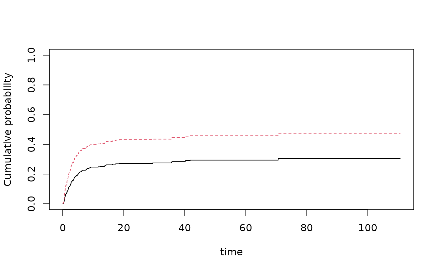
nd <- data.frame(tcell=c(1,0),platelet=0,age=0)
por <- predict(or,nd)
plot(por)


## approximate standard errors 
por <-mets:::predict.phreg(or,nd)
plot(por,se=1)

## Fine-Gray model
fg=cifregFG(Event(time,cause)~tcell+platelet+age,data=bmt,cause=1)
summary(fg)
#> 
#>    n events
#>  408    161
#> 
#>  408 clusters
#> coefficients:
#>           Estimate      S.E.   dU^-1/2 P-value
#> tcell    -0.597055  0.270452  0.275783  0.0273
#> platelet -0.426037  0.180707  0.187720  0.0184
#> age       0.343921  0.080270  0.086285  0.0000
#> 
#> exp(coefficients):
#>          Estimate    2.5%  97.5%
#> tcell     0.55043 0.32396 0.9352
#> platelet  0.65309 0.45831 0.9307
#> age       1.41047 1.20514 1.6508
#> 
##fg=recreg(Event(time,cause)~tcell+platelet+age,data=bmt,cause=1,death.code=2)
##summary(fg)
plot(fg)

nd <- data.frame(tcell=c(1,0),platelet=0,age=0)
pfg <- predict(fg,nd,se=1)
plot(pfg,se=1)

## bt <- iidBaseline(fg,time=30)
## bt <- IIDrecreg(fg$cox.prep,fg,time=30)

## not run to avoid timing issues
## gofFG(Event(time,cause)~tcell+platelet+age,data=bmt,cause=1)

sfg <- cifregFG(Event(time,cause)~strata(tcell)+platelet+age,data=bmt,cause=1)
summary(sfg)
#> 
#>    n events
#>  408    161
#> 
#>  408 clusters
#> coefficients:
#>           Estimate      S.E.   dU^-1/2 P-value
#> platelet -0.424645  0.180792  0.187822  0.0188
#> age       0.342094  0.079862  0.086285  0.0000
#> 
#> exp(coefficients):
#>          Estimate    2.5%  97.5%
#> platelet  0.65400 0.45887 0.9321
#> age       1.40789 1.20390 1.6465
#> 
plot(sfg)


### predictions with CI based on iid decomposition of baseline and beta
### these are used in the predict function above
fg <- cifregFG(Event(time,cause)~tcell+platelet+age,data=bmt,cause=1)
Biid <- iidBaseline(fg,time=20)
pfg1 <- FGprediid(Biid,nd)
pfg1
#>           pred     se-log     lower     upper
#> [1,] 0.2692822 0.22756923 0.1723853 0.4206442
#> [2,] 0.4344567 0.07477993 0.3752267 0.5030363