Marginal mean estimation for recurrent events with a terminal event

Estimates the marginal mean number of recurrent events over time in the presence of a competing terminal event (e.g. death), using the nonparametric estimator of Ghosh and Lin (2000). Two proportional hazards models are fitted internally—one for the recurrent event rate and one for the terminal event—and combined to form the estimator $$\mu(t) = \int_0^t S(u-)\,dR(u),$$ where $S(u)$ is the marginal survival probability at the baseline covariate level and $dR(u)$ is the baseline recurrent event rate among survivors. Robust (sandwich) standard errors are computed via the influence-function approach of Ghosh and Lin (2000).

Usage

recurrent_marginal(formula, data, cause = 1, ..., death.code = 2, test = FALSE)

recurrentMarginal(formula, data, ...)

Arguments

formula: A formula with an Event response on the left-hand side, specifying entry time, exit time, and event status. The right-hand side may include cluster() to identify subjects and strata() for a stratified analysis. A cluster() term is required.
data: A data frame containing all variables in formula.
cause: Integer code(s) for the recurrent event of interest. Default is 1.
...: Further arguments passed to phreg.
death.code: Integer code(s) for the terminal event. Default is 2.
test: Logical. If TRUE, a logrank-type test comparing strata is computed and stored as an attribute of the result. Default is FALSE.

Value

An object of class "recurrent" with the following components:

mu: Estimated marginal mean $\mu(t)$ at each jump time.
se.mu: Robust standard error of mu.
times: Jump times at which estimates are computed.
St: Marginal survival estimate $S(t)$ at each jump time.
cumhaz: Two-column matrix of (time, mu), suitable for plotting.
se.cumhaz: Two-column matrix of (time, se.mu).

The object carries three attributes: "logrank" (the test result when test = TRUE, otherwise NULL), "cause", and "death.code".

Details

Jump times must be unique within each stratum. If ties are present, use tie_breaker to resolve them before calling this function.

References

Cook, R. J. and Lawless, J. F. (1997). Marginal analysis of recurrent events and a terminating event. Statistics in Medicine, 16, 911–924.

Ghosh, D. and Lin, D. Y. (2000). Nonparametric analysis of recurrent events and death. Biometrics, 56, 554–562.

Author

Thomas Scheike

Examples

data(hfactioncpx12)
hf <- hfactioncpx12
hf$x <- as.numeric(hf$treatment)

## Fit nonparametric baseline models for recurrent events and death
xr <- phreg(Surv(entry, time, status == 1) ~ cluster(id), data = hf)
dr <- phreg(Surv(entry, time, status == 2) ~ cluster(id), data = hf)

par(mfrow = c(1, 3))
plot(dr, se = TRUE); title(main = "Death")
plot(xr, se = TRUE); title(main = "Recurrent events")

## Compare naive and robust standard errors for the recurrent event rate
rxr <- robust_phreg(xr, fixbeta = 1)
plot(rxr, se = TRUE, robust = TRUE, add = TRUE, col = 4)

## Marginal mean via formula interface
outN <- recurrent_marginal(Event(entry, time, status) ~ cluster(id),
                           data = hf, cause = 1, death.code = 2)
plot(outN, se = TRUE, col = 2, add = TRUE)
summary(outN, times = 1:5)
#> [[1]]
#>        new.time      mean         se   CI-2.5% CI-97.5% strata
#> 608           1 0.8282358 0.04844543 0.7385251 0.928844      0
#> 1053          2 1.5139493 0.07039884 1.3820710 1.658412      0
#> 1282          3 2.0244982 0.08351867 1.8672476 2.194992      0
#> 1392          4 2.5004732 0.10843166 2.2967320 2.722288      0
#> 1392.1        5 2.5004732 0.10843166 2.2967320 2.722288      0
#> 

## Stratified analysis with logrank test
out <- recurrent_marginal(Event(entry, time, status) ~ strata(treatment) + cluster(id),
                          data = hf, cause = 1, death.code = 2, test = TRUE)
plot(out, se = TRUE, ylab = "Marginal mean", col = 1:2)

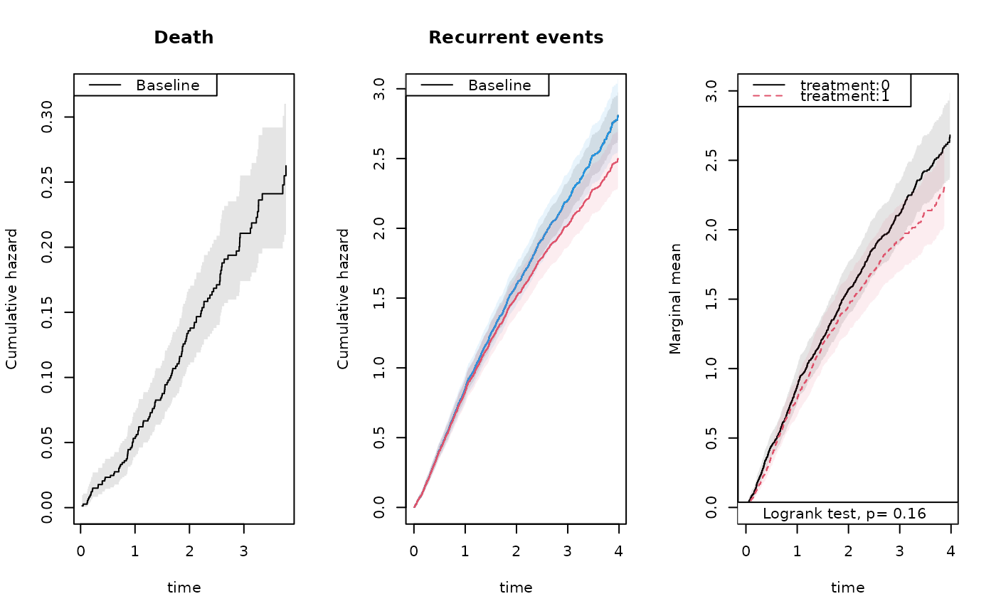attr(out, "logrank")
#>    Estimate Std.Err   2.5% 97.5% P-value
#> p1    37.98   27.04 -15.01 90.97  0.1601
#> ────────────────────────────────────────────────────────────
#> Null Hypothesis: 
#>   [p1] = 0 
#>  
#> chisq = 1.9737, df = 1, p-value = 0.1601
summary(out, times = 1:5)
#> [[1]]
#>       new.time      mean         se   CI-2.5% CI-97.5% strata
#> 325          1 0.8737156 0.06783343 0.7503858 1.017315      0
#> 555          2 1.5718563 0.09572955 1.3949953 1.771140      0
#> 682          3 2.1184963 0.11385721 1.9066915 2.353829      0
#> 748          4 2.6815219 0.15451005 2.3951619 3.002118      0
#> 748.1        5 2.6815219 0.15451005 2.3951619 3.002118      0
#> 
#> [[2]]
#>       new.time      mean         se   CI-2.5%  CI-97.5% strata
#> 284          1 0.7815557 0.06908585 0.6572305 0.9293989      1
#> 499          2 1.4534055 0.10315606 1.2646561 1.6703258      1
#> 601          3 1.9240624 0.12165771 1.6998008 2.1779119      1
#> 645          4 2.3134997 0.14963892 2.0380418 2.6261880      1
#> 645.1        5 2.3134997 0.14963892 2.0380418 2.6261880      1
#> 

## Influence-function (iid) decomposition at a fixed time point
head(iid(outN, time = 3))
#>         strata0
#> 1  2.547554e-04
#> 2  6.537407e-04
#> 3  4.236127e-03
#> 4 -1.378931e-03
#> 5 -5.105272e-05
#> 6 -3.424693e-03