Simulation of output from Cumulative incidence regression model
Source:R/sim-pc-hazard.R
sim.cif.RdSimulates data that looks like fit from fitted cumulative incidence model
Usage
sim.cif(
  cif,
  n,
  data = NULL,
  Z = NULL,
  rr = NULL,
  strata = NULL,
  drawZ = TRUE,
  cens = NULL,
  rrc = NULL,
  cumstart = c(0, 0),
  U = NULL,
  pU = NULL,
  type = NULL,
  extend = NULL,
  ...
)
Arguments
- cif
output form prop.odds.subdist or ccr (cmprsk), can also call invsubdist with with cumulative and linear predictor
- n
number of simulations.
- data
to extract covariates for simulations (draws from observed covariates).
- Z
to use these covariates for simulation rather than drawing new ones.
- rr
possible vector of relative risk for cox model.
- strata
possible vector of strata
- drawZ
to random sample from Z or not
- cens
specifies censoring model, if "is.matrix" then uses cumulative hazard given, if "is.scalar" then uses rate for exponential, and if not given then takes average rate of in simulated data from cox model.
- rrc
possible vector of relative risk for cox-type censoring.
- cumstart
to start cumulatives at time 0 in 0.
- U
uniforms to use for drawing of timing for cumulative incidence.
- pU
uniforms to use for drawing event type (F1,F2,1-F1-F2).
- type
of model logistic,cloglog,rr
- extend
to extend piecewise constant with constant rate. Default is average rate over time from cumulative (when TRUE), if numeric then uses given rate.
- ...
arguments for simsubdist (for example Uniform variable for realizations)
Examples
library(mets)
data(bmt)
nsim <- 100
## logit cumulative incidence regression model
cif <- cifreg(Event(time,cause)~platelet+age,data=bmt,cause=1)
estimate(cif)
#> Estimate Std.Err 2.5% 97.5% P-value
#> platelet -0.5300 0.23329 -0.9873 -0.07275 0.0230973
#> age 0.3553 0.09611 0.1669 0.54365 0.0002187
plot(cif,col=1)
simbmt <- sim.cif(cif,nsim,data=bmt)
dtable(simbmt,~status)
#>
#> status
#> 0 1
#> 62 38
#>
scif <- cifreg(Event(time,status)~platelet+age,data=simbmt,cause=1)
estimate(scif)
#> Estimate Std.Err 2.5% 97.5% P-value
#> platelet 0.1401 0.4363 -0.7150 0.9953 0.74808
#> age 0.4783 0.2072 0.0722 0.8843 0.02097
plot(scif,add=TRUE,col=2)
 ## Fine-Gray cloglog cumulative incidence regression model
cif <- cifregFG(Event(time,cause)~strata(tcell)+age,data=bmt,cause=1)
estimate(cif)
#> Estimate Std.Err 2.5% 97.5% P-value
#> age 0.3584 0.07883 0.2039 0.5129 5.469e-06
plot(cif,col=1)
simbmt <- sim.cif(cif,nsim,data=bmt)
scif <- cifregFG(Event(time,status)~strata(tcell)+age,data=simbmt,cause=1)
estimate(scif)
#> Estimate Std.Err 2.5% 97.5% P-value
#> age 0.3866 0.1936 0.007124 0.7661 0.04585
plot(scif,add=TRUE,col=2)
## Fine-Gray cloglog cumulative incidence regression model
cif <- cifregFG(Event(time,cause)~strata(tcell)+age,data=bmt,cause=1)
estimate(cif)
#> Estimate Std.Err 2.5% 97.5% P-value
#> age 0.3584 0.07883 0.2039 0.5129 5.469e-06
plot(cif,col=1)
simbmt <- sim.cif(cif,nsim,data=bmt)
scif <- cifregFG(Event(time,status)~strata(tcell)+age,data=simbmt,cause=1)
estimate(scif)
#> Estimate Std.Err 2.5% 97.5% P-value
#> age 0.3866 0.1936 0.007124 0.7661 0.04585
plot(scif,add=TRUE,col=2)
 ################################################################
# simulating several causes with specific cumulatives
################################################################
cif1 <- cifreg(Event(time,cause)~strata(tcell)+age,data=bmt,cause=1)
cif2 <- cifreg(Event(time,cause)~strata(platelet)+tcell+age,data=bmt,cause=2)
cifss <- list(cif1,cif2)
simbmt <- sim.cifs(list(cif1,cif2),nsim,data=bmt,extend=0.005)
dtable(simbmt,~status)
#>
#> status
#> 0 1 2
#> 49 41 10
#>
scif1 <- cifreg(Event(time,status)~strata(tcell)+age,data=simbmt,cause=1)
scif2 <- cifreg(Event(time,status)~strata(platelet)+tcell+age,data=simbmt,cause=2)
cbind(cif1$coef,scif1$coef)
#> [,1] [,2]
#> age 0.4157306 0.6036799
## can be off due to restriction F1+F2<= 1
cbind(cif2$coef,scif2$coef)
#> [,1] [,2]
#> tcell 0.68379711 1.2507661
#> age -0.03484497 0.9837646
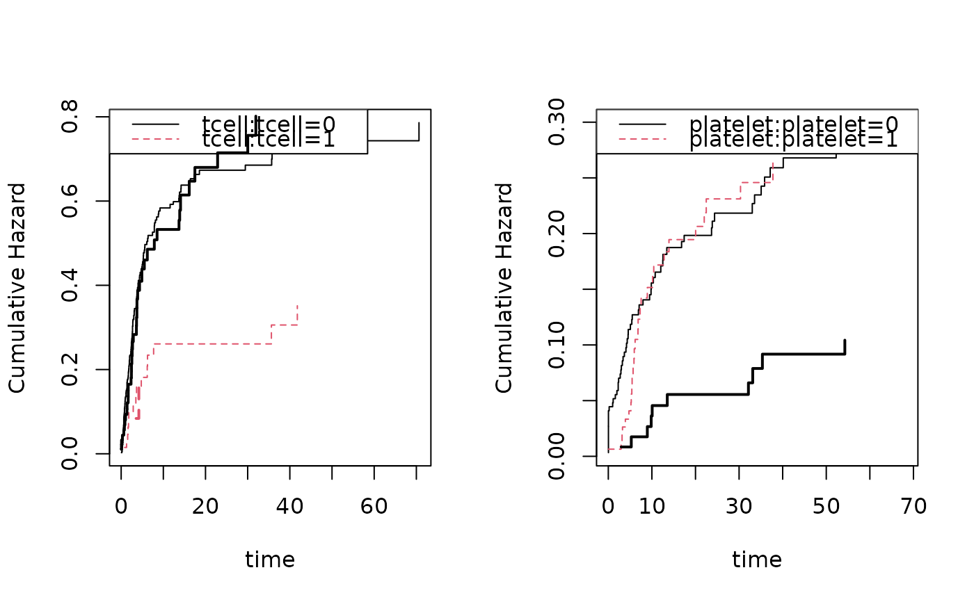
par(mfrow=c(1,2))
## Cause 1 follows the model
plot(cif1); plot(scif1,add=TRUE,col=1:2,lwd=2)
# Cause 2:second cause is modified with restriction to satisfy F1+F2<= 1, so scaled down
plot(cif2); plot(scif2,add=TRUE,col=1:2,lwd=2)
################################################################
# simulating several causes with specific cumulatives
################################################################
cif1 <- cifreg(Event(time,cause)~strata(tcell)+age,data=bmt,cause=1)
cif2 <- cifreg(Event(time,cause)~strata(platelet)+tcell+age,data=bmt,cause=2)
cifss <- list(cif1,cif2)
simbmt <- sim.cifs(list(cif1,cif2),nsim,data=bmt,extend=0.005)
dtable(simbmt,~status)
#>
#> status
#> 0 1 2
#> 49 41 10
#>
scif1 <- cifreg(Event(time,status)~strata(tcell)+age,data=simbmt,cause=1)
scif2 <- cifreg(Event(time,status)~strata(platelet)+tcell+age,data=simbmt,cause=2)
cbind(cif1$coef,scif1$coef)
#> [,1] [,2]
#> age 0.4157306 0.6036799
## can be off due to restriction F1+F2<= 1
cbind(cif2$coef,scif2$coef)
#> [,1] [,2]
#> tcell 0.68379711 1.2507661
#> age -0.03484497 0.9837646
par(mfrow=c(1,2))
## Cause 1 follows the model
plot(cif1); plot(scif1,add=TRUE,col=1:2,lwd=2)
# Cause 2:second cause is modified with restriction to satisfy F1+F2<= 1, so scaled down
plot(cif2); plot(scif2,add=TRUE,col=1:2,lwd=2)