Discrete Time-to-Event Analysis with Interval Censoring
Source:R/interval-cumoddsreg.r
interval_logitsurv_discrete.RdFits a cumulative odds model for discrete time-to-event data, handling interval censoring where the event time is known only to lie within an interval \((t_l, t_r]\). The model assumes: $$ \text{logit}(P(T \leq t | x)) = \log(G(t)) + x \beta $$ where \(G(t)\) is the baseline cumulative odds function and \(\beta\) are the regression coefficients. This is equivalent to: $$ P(T \leq t | x) = \frac{G(t) \exp(x \beta)}{1 + G(t) \exp(x \beta)} $$
Usage
interval_logitsurv_discrete(
  formula,
  data,
  beta = NULL,
  no.opt = FALSE,
  method = "NR",
  stderr = TRUE,
  weights = NULL,
  offsets = NULL,
  exp.link = 1,
  increment = 1,
  ...
)
Arguments
- formula
Formula with an
Intervalobject (e.g.,Interval(entry, time)) on the left-hand side and covariates on the right. Can includecluster()for correlated data.- data
Data frame containing the variables in the formula.
- beta
Starting values for the optimization (vector of length \(p + k\), where \(p\) is the number of covariates and \(k\) is the number of time intervals).
- no.opt
Logical; if TRUE, skips optimization and returns estimates based on the provided
beta(useful for initialization).- method
Optimization method:
"NR"(Newton-Raphson, default) or"nlm".- stderr
Logical; if FALSE, returns only the coefficient estimates.
- weights
Observation weights (follows ID).
- offsets
Offsets (follows ID).
- exp.link
Logical; if TRUE, parameterizes increments as \(\exp(\alpha) > 0\).
- increment
Logical; if TRUE, uses increments \(dG(t) = \exp(\alpha)\) as parameters.
- ...
Additional arguments passed to the optimizer (
lava::NRornlm).
Value
An object of class "cumoddsreg" containing:
- coef
Estimated coefficients (baseline time effects and covariate effects).
- se.coef
Standard errors of the coefficients.
- var
Variance-covariance matrix.
- iid
Influence function (IID) decomposition for robust variance estimation.
- ntimes
Number of distinct time intervals.
- utimes
Unique time points.
- ploglik
Log-likelihood at convergence.
- gradient, hessian
Optimization results.
- call
Original function call.
Details
The baseline \(G(t)\) is parameterized as the cumulative sum of exponentials (\(G(t) = \sum \exp(\alpha)\)), ensuring positivity. The regression coefficients describe the log-odds of the event occurring by time \(t\).
The likelihood is maximized over the observed intervals: $$ L = \prod_i [ P(T_i > t_{il} | x_i) - P(T_i > t_{ir} | x_i) ] $$ where \(t_{il}\) and \(t_{ir}\) are the left and right endpoints of the interval for subject \(i\). Right-censored intervals have \(t_{ir} = \infty\).
References
Scheike, T. H. (2024). Discrete time survival analysis with interval censoring. mets package documentation.
See also
cumoddsreg, predictlogitSurvd, simlogitSurvd
Examples
data(ttpd)
dtable(ttpd,~entry+time2)
#>
#> time2 1 2 3 4 5 6 Inf
#> entry
#> 0 316 0 0 0 0 0 0
#> 1 0 133 0 0 0 0 0
#> 2 0 0 150 0 0 0 0
#> 3 0 0 0 23 0 0 0
#> 4 0 0 0 0 90 0 0
#> 5 0 0 0 0 0 68 0
#> 6 0 0 0 0 0 0 220
out <- interval_logitsurv_discrete(Interval(entry,time2)~X1+X2+X3+X4,ttpd)
summary(out)
#> $baseline
#> Estimate Std.Err 2.5% 97.5% P-value
#> time1 -2.0064 0.1523 -2.305 -1.7079 1.273e-39
#> time2 -2.1749 0.1599 -2.488 -1.8614 4.118e-42
#> time3 -1.4581 0.1544 -1.761 -1.1554 3.636e-21
#> time4 -2.9260 0.2453 -3.407 -2.4453 8.379e-33
#> time5 -1.2051 0.1706 -1.539 -0.8706 1.633e-12
#> time6 -0.9102 0.1860 -1.275 -0.5457 9.843e-07
#>
#> $logor
#> Estimate Std.Err 2.5% 97.5% P-value
#> X1 0.9913 0.1179 0.76024 1.2223 4.100e-17
#> X2 0.6962 0.1162 0.46847 0.9238 2.064e-09
#> X3 0.3466 0.1159 0.11941 0.5738 2.788e-03
#> X4 0.3223 0.1151 0.09668 0.5478 5.111e-03
#>
#> $or
#> Estimate 2.5% 97.5%
#> X1 2.694610 2.138791 3.394874
#> X2 2.006032 1.597554 2.518953
#> X3 1.414239 1.126834 1.774950
#> X4 1.380231 1.101503 1.729490
#>
head(iid(out))
#> [,1] [,2] [,3] [,4] [,5]
#> 1 0.0045687959 0.004769499 0.0053427163 0.0059138018 0.0066308444
#> 2 0.0016959549 0.002038630 0.0025477402 0.0029776943 -0.0102830496
#> 3 0.0045687959 0.004769499 0.0053427163 0.0059138018 0.0066308444
#> 4 0.0027545442 -0.006047556 -0.0007244072 -0.0006949805 -0.0006704063
#> 5 -0.0002919658 -0.008889214 -0.0026820744 -0.0026532556 -0.0026268232
#> 6 0.0001497624 -0.008530642 -0.0033151419 -0.0032325395 -0.0031636812
#> [,6] [,7] [,8] [,9] [,10]
#> 1 0.0081721788 -0.0033482398 -0.0034168560 0.0034308192 -0.0034212419
#> 2 -0.0012875717 -0.0007883982 -0.0005310631 -0.0004080546 -0.0000776067
#> 3 0.0081721788 -0.0033482398 -0.0034168560 0.0034308192 -0.0034212419
#> 4 -0.0006379316 0.0003557924 0.0007697270 0.0008855193 -0.0013506040
#> 5 -0.0025608456 -0.0026170215 0.0016772465 0.0020412533 0.0017043055
#> 6 -0.0030621110 0.0015290328 0.0016662399 0.0020179143 0.0017471657
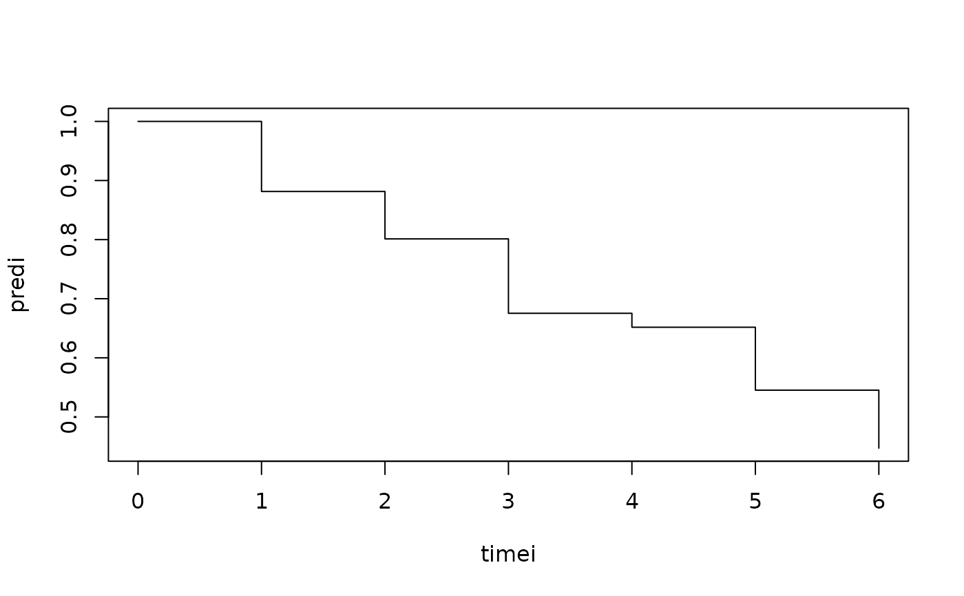
pred <- predictlogitSurvd(out,se=FALSE)
plotSurvd(pred)
 ttpd <- dfactor(ttpd,fentry~entry)
out <- cumoddsreg(fentry~X1+X2+X3+X4,ttpd)
summary(out)
#> $baseline
#> Estimate Std.Err 2.5% 97.5% P-value
#> time1 -2.0064 0.1523 -2.305 -1.7079 1.273e-39
#> time2 -2.1749 0.1599 -2.488 -1.8614 4.118e-42
#> time3 -1.4581 0.1544 -1.761 -1.1554 3.636e-21
#> time4 -2.9260 0.2453 -3.407 -2.4453 8.379e-33
#> time5 -1.2051 0.1706 -1.539 -0.8706 1.633e-12
#> time6 -0.9102 0.1860 -1.275 -0.5457 9.843e-07
#>
#> $logor
#> Estimate Std.Err 2.5% 97.5% P-value
#> X1 0.9913 0.1179 0.76024 1.2223 4.100e-17
#> X2 0.6962 0.1162 0.46847 0.9238 2.064e-09
#> X3 0.3466 0.1159 0.11941 0.5738 2.788e-03
#> X4 0.3223 0.1151 0.09668 0.5478 5.111e-03
#>
#> $or
#> Estimate 2.5% 97.5%
#> X1 2.694610 2.138791 3.394874
#> X2 2.006032 1.597554 2.518953
#> X3 1.414239 1.126834 1.774950
#> X4 1.380231 1.101503 1.729490
#>
ttpd <- dfactor(ttpd,fentry~entry)
out <- cumoddsreg(fentry~X1+X2+X3+X4,ttpd)
summary(out)
#> $baseline
#> Estimate Std.Err 2.5% 97.5% P-value
#> time1 -2.0064 0.1523 -2.305 -1.7079 1.273e-39
#> time2 -2.1749 0.1599 -2.488 -1.8614 4.118e-42
#> time3 -1.4581 0.1544 -1.761 -1.1554 3.636e-21
#> time4 -2.9260 0.2453 -3.407 -2.4453 8.379e-33
#> time5 -1.2051 0.1706 -1.539 -0.8706 1.633e-12
#> time6 -0.9102 0.1860 -1.275 -0.5457 9.843e-07
#>
#> $logor
#> Estimate Std.Err 2.5% 97.5% P-value
#> X1 0.9913 0.1179 0.76024 1.2223 4.100e-17
#> X2 0.6962 0.1162 0.46847 0.9238 2.064e-09
#> X3 0.3466 0.1159 0.11941 0.5738 2.788e-03
#> X4 0.3223 0.1151 0.09668 0.5478 5.111e-03
#>
#> $or
#> Estimate 2.5% 97.5%
#> X1 2.694610 2.138791 3.394874
#> X2 2.006032 1.597554 2.518953
#> X3 1.414239 1.126834 1.774950
#> X4 1.380231 1.101503 1.729490
#>