Calibration for multiclassication methods
Usage
calibration(
  pr,
  cl,
  weights = NULL,
  threshold = 10,
  method = "bin",
  breaks = nclass.Sturges,
  df = 3,
  ...
)
Arguments
- pr
matrix with probabilities for each class
- cl
class variable
- weights
counts
- threshold
do not calibrate if less then 'threshold' events
- method
either 'isotonic' (pava), 'logistic', 'mspline' (monotone spline), 'bin' (local constant)
- breaks
optional number of bins (only for method 'bin')
- df
degrees of freedom (only for spline methods)
- ...
additional arguments to lower level functions
Value
An object of class 'calibration' is returned.
See calibration-class
for more details about this class and its generic functions.
Examples
sim1 <- function(n, beta=c(-3, rep(.5,10)), rho=.5) {
p <- length(beta)-1
xx <- lava::rmvn0(n,sigma=diag(nrow=p)*(1-rho)+rho)
y <- rbinom(n, 1, lava::expit(cbind(1,xx)%*%beta))
d <- data.frame(y=y, xx)
names(d) <- c("y",paste0("x",1:p))
return(d)
}
set.seed(1)
beta <- c(-2,rep(1,10))
d <- sim1(1e4, beta=beta)
a1 <- naivebayes(y ~ ., data=d)
a2 <- glm(y ~ ., data=d, family=binomial)
#> Warning: glm.fit: fitted probabilities numerically 0 or 1 occurred
## a3 <- randomForest(factor(y) ~ ., data=d, family=binomial)
d0 <- sim1(1e4, beta=beta)
p1 <- predict(a1, newdata=d0)
p2 <- predict(a2, newdata=d0, type="response")
## p3 <- predict(a3, newdata=d0, type="prob")
c2 <- calibration(p2, d0$y, method="isotonic")
c1 <- calibration(p1, d0$y, breaks=100)
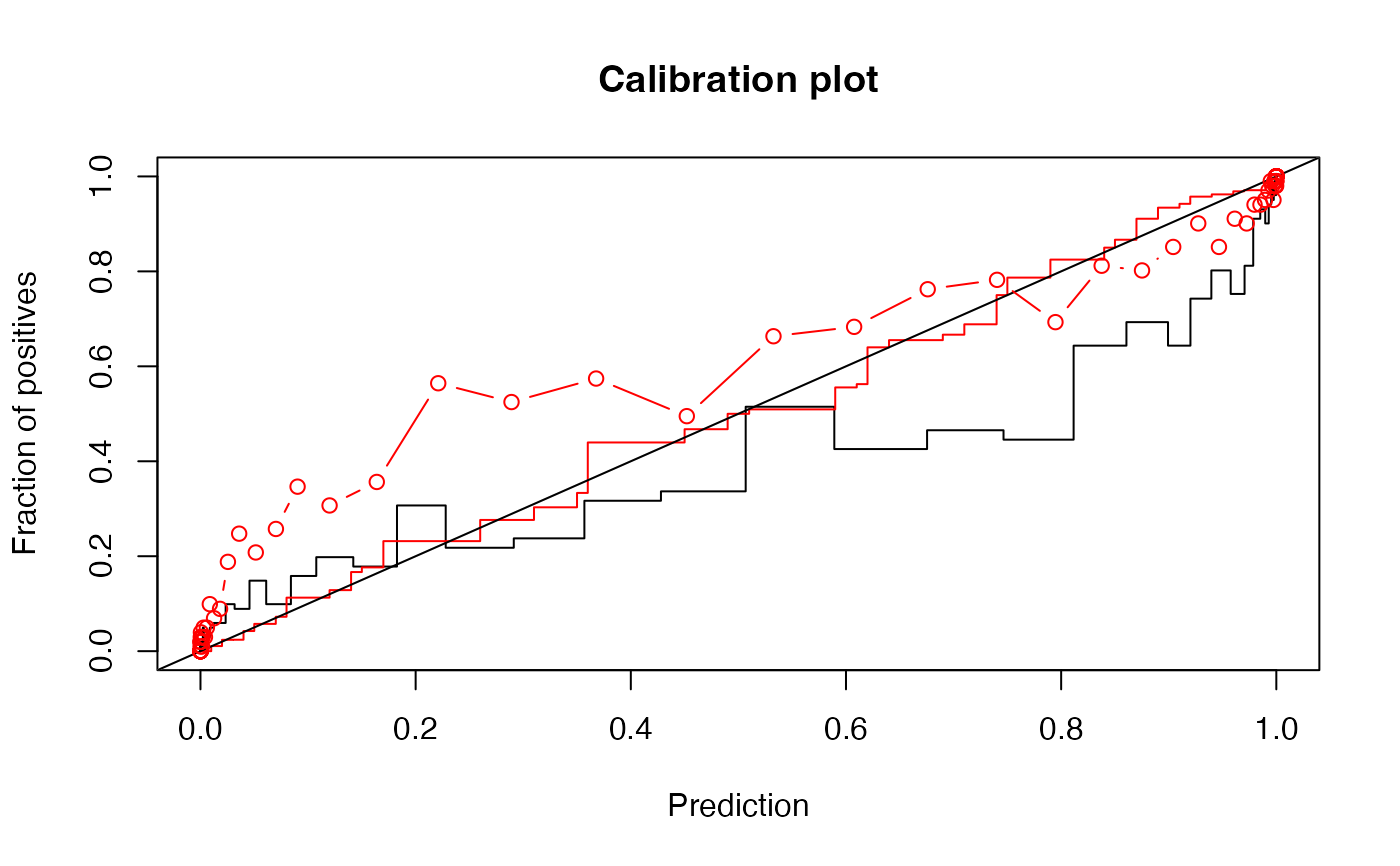
if (interactive()) {
plot(c1)
plot(c2,col="red",add=TRUE)
abline(a=0,b=1)
with(c1$xy[[1]], points(pred,freq,type="b", col="red"))
}
 set.seed(1)
beta <- c(-2,rep(1,10))
dd <- lava::csplit(sim1(1e4, beta=beta), k=3)
mod <- naivebayes(y ~ ., data=dd[[1]])
p1 <- predict(mod, newdata=dd[[2]])
cal <- calibration(p1, dd[[2]]$y)
p2 <- predict(mod, newdata=dd[[3]])
pp <- predict(c1, p2)
cc <- calibration(pp, dd[[3]]$y)
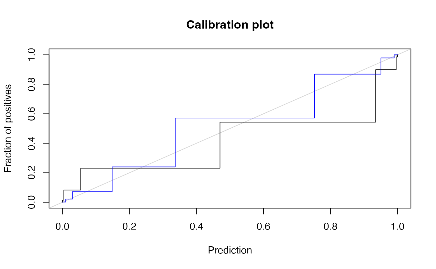
if (interactive()) {#'
plot(cal)
plot(cc, add=TRUE, col="blue")
}
set.seed(1)
beta <- c(-2,rep(1,10))
dd <- lava::csplit(sim1(1e4, beta=beta), k=3)
mod <- naivebayes(y ~ ., data=dd[[1]])
p1 <- predict(mod, newdata=dd[[2]])
cal <- calibration(p1, dd[[2]]$y)
p2 <- predict(mod, newdata=dd[[3]])
pp <- predict(c1, p2)
cc <- calibration(pp, dd[[3]]$y)
if (interactive()) {#'
plot(cal)
plot(cc, add=TRUE, col="blue")
}