Regression model for binomial data with unkown group of immortals (zero-inflated binomial regression)
Usage
zibreg(
  formula,
  formula.p = ~1,
  data,
  family = stats::binomial(),
  offset = NULL,
  start,
  var = "hessian",
  ...
)
Arguments
- formula
Formula specifying
- formula.p
Formula for model of disease prevalence
- data
data frame
- family
Distribution family (see the help page
family)- offset
Optional offset
- start
Optional starting values
- var
Type of variance (robust, expected, hessian, outer)
- ...
Additional arguments to lower level functions
Examples
## Simulation
n <- 2e3
x <- runif(n,0,20)
age <- runif(n,10,30)
z0 <- rnorm(n,mean=-1+0.05*age)
z <- cut(z0,breaks=c(-Inf,-1,0,1,Inf))
p0 <- lava:::expit(model.matrix(~z+age) %*% c(-.4, -.4, 0.2, 2, -0.05))
y <- (runif(n)<lava:::tigol(-1+0.25*x-0*age))*1
u <- runif(n)<p0
y[u==0] <- 0
d <- data.frame(y=y,x=x,u=u*1,z=z,age=age)
head(d)
#> y x u z age
#> 1 1 11.563238 1 (0,1] 29.90851
#> 2 0 19.742035 0 (0,1] 25.19084
#> 3 1 12.075848 1 (0,1] 19.42130
#> 4 0 1.298998 0 (-1,0] 15.15169
#> 5 0 3.242182 0 (-Inf,-1] 17.67022
#> 6 0 9.507958 0 (-1,0] 15.95907
## Estimation
e0 <- zibreg(y~x*z,~1+z+age,data=d)
e <- zibreg(y~x,~1+z+age,data=d)
compare(e,e0)
#>
#> - Likelihood ratio test -
#>
#> data:
#> chisq = 11.003, df = 6, p-value = 0.08827
#> sample estimates:
#> log likelihood (model 1) log likelihood (model 2)
#> -878.7915 -873.2898
#>
e
#> Estimate 2.5% 97.5% P-value
#> (Intercept) -0.92653261 -1.45236281 -0.40070241 5.533001e-04
#> x 0.24651707 0.10557819 0.38745596 6.076311e-04
#> pr:(Intercept) -0.05222810 -0.62292225 0.51846604 8.576475e-01
#> pr:z(-1,0] -0.56082650 -0.95643238 -0.16522062 5.460677e-03
#> pr:z(0,1] 0.04696480 -0.33424353 0.42817312 8.091930e-01
#> pr:z(1, Inf] 1.91101695 1.42311752 2.39891638 1.630647e-14
#> pr:age -0.06280124 -0.08717892 -0.03842355 4.436302e-07
#>
#> Prevalence probabilities:
#> Estimate 2.5% 97.5%
#> {(Intercept)} 0.4869459 0.3491171 0.6267890
#> {(Intercept)} + {z(-1,0]} 0.3513627 0.2364406 0.4865494
#> {(Intercept)} + {z(0,1]} 0.4986842 0.3526182 0.6449751
#> {(Intercept)} + {z(1, Inf]} 0.8651557 0.7433110 0.9342773
#> {(Intercept)} + {age} 0.4712743 0.3392018 0.6074950
PD(e0,intercept=c(1,3),slope=c(2,6))
#> Estimate Std.Err 2.5% 97.5%
#> 50% 4.257552 1.519033 1.280302 7.234802
#> attr(,"b")
#> [1] -1.8332904 0.4305973
B <- rbind(c(1,0,0,0,20),
c(1,1,0,0,20),
c(1,0,1,0,20),
c(1,0,0,1,20))
prev <- summary(e,pr.contrast=B)$prevalence
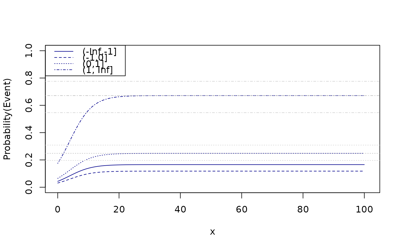
x <- seq(0,100,length.out=100)
newdata <- expand.grid(x=x,age=20,z=levels(d$z))
fit <- predict(e,newdata=newdata)
plot(0,0,type="n",xlim=c(0,101),ylim=c(0,1),xlab="x",ylab="Probability(Event)")
count <- 0
for (i in levels(newdata$z)) {
count <- count+1
lines(x,fit[which(newdata$z==i)],col="darkblue",lty=count)
}
abline(h=prev[3:4,1],lty=3:4,col="gray")
abline(h=prev[3:4,2],lty=3:4,col="lightgray")
abline(h=prev[3:4,3],lty=3:4,col="lightgray")
legend("topleft",levels(d$z),col="darkblue",lty=seq_len(length(levels(d$z))))