Fits a Cox proportional hazards model using a fast C++ backend. Robust variance (sandwich estimator) is the default variance estimate in the summary.
Value
An object of class "phreg" containing:
- coef
Vector of estimated coefficients.
- var
Robust variance-covariance matrix.
- beta.iid
Influence functions for the regression coefficients.
- cumhaz
Matrix of cumulative hazard estimates (time, cumhaz).
- se.cumhaz
Matrix of standard errors for the cumulative hazard.
- cox.prep
List containing preprocessed data for the Cox model.
- opt
Optimization results (if optimization was performed).
- call
The matched call.
Details
The influence functions (IID decomposition) follow the numerical order of the given cluster variable. Ordering the results by `$id` will align the IID terms with the original dataset order.
See also
plot.phreg, predict.phreg, robust_phreg
Examples
data(TRACE)
dcut(TRACE) <- ~.
# Fit model with clustering
out1 <- phreg(Surv(time, status == 9) ~ wmi + age + strata(vf, chf) + cluster(id), data = TRACE)
summary(out1)
#>
#> n events
#> 1878 958
#> coefficients:
#> Estimate S.E. dU^-1/2 P-value
#> wmi -0.8470690 0.0871082 0.0864370 0
#> age 0.0563491 0.0037111 0.0036386 0
#>
#> exp(coefficients):
#> Estimate 2.5% 97.5%
#> wmi 0.42867 0.36139 0.5085
#> age 1.05797 1.05030 1.0657
#>
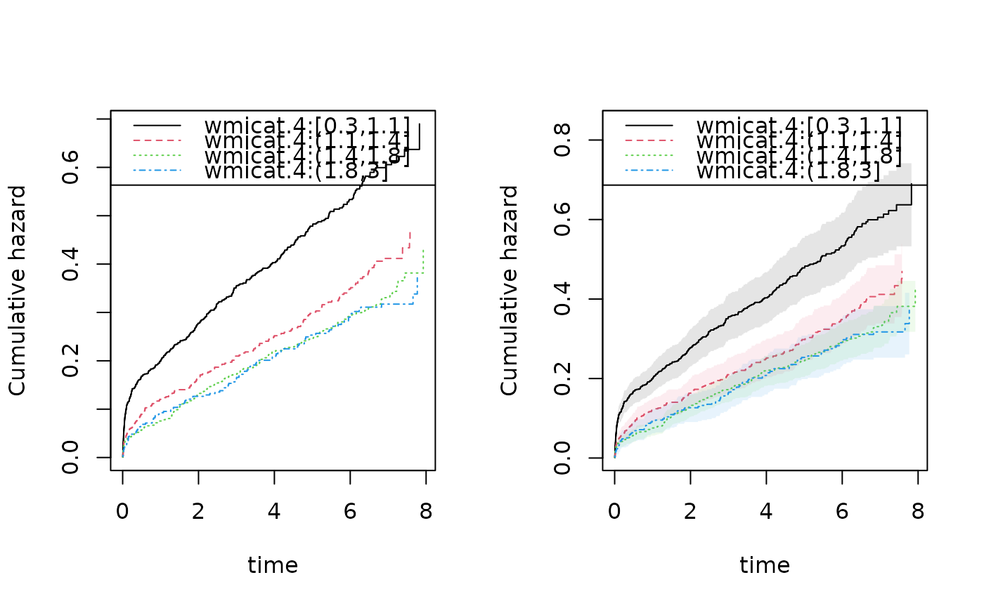
# Plotting baselines
par(mfrow = c(1, 2))
plot(out1)
# Computing robust variance for baseline
rob1 <- robust_phreg(out1)
plot(rob1, se = TRUE, robust = TRUE)
 # IID decomposition for regression parameters
head(iid(out1))
#> wmi age
#> 3 2.315573e-04 8.113514e-05
#> 7 -1.175364e-03 -2.901628e-05
#> 13 1.826339e-03 1.670430e-04
#> 15 -3.739823e-05 2.673793e-05
#> 17 -2.997039e-03 5.371497e-05
#> 22 -9.146118e-04 -9.342247e-06
# IID decomposition for baseline at a specific time-point
Aiiid <- iid(out1, time = 30)
head(Aiiid)
#> strata0 strata1 strata2 strata3
#> 3 -1.894877e-04 -4.120570e-04 -2.659857e-04 -7.350908e-04
#> 7 1.812767e-04 2.367745e-04 1.678711e-04 8.774722e-04
#> 13 -6.837818e-04 -1.063129e-03 -6.374803e-04 -1.717426e-03
#> 15 -8.543458e-05 -9.149095e-05 -8.008394e-05 -2.250601e-04
#> 17 4.118052e-05 3.243790e-05 3.366936e-05 -1.046447e-05
#> 22 5.011669e-05 1.201129e-04 8.975026e-05 2.188617e-04
# Combined IID decomposition (beta and baseline)
dd <- iidBaseline(out1, time = 30)
head(dd$beta.iid)
#> [,1] [,2]
#> 3 2.315573e-04 8.113514e-05
#> 7 -1.175364e-03 -2.901628e-05
#> 13 1.826339e-03 1.670430e-04
#> 15 -3.739823e-05 2.673793e-05
#> 17 -2.997039e-03 5.371497e-05
#> 22 -9.146118e-04 -9.342247e-06
head(dd$base.iid)
#> strata0 strata1 strata2 strata3
#> 3 -1.894877e-04 -4.120570e-04 -2.659857e-04 -7.350908e-04
#> 7 1.812767e-04 2.367745e-04 1.678711e-04 8.774722e-04
#> 13 -6.837818e-04 -1.063129e-03 -6.374803e-04 -1.717426e-03
#> 15 -8.543458e-05 -9.149095e-05 -8.008394e-05 -2.250601e-04
#> 17 4.118052e-05 3.243790e-05 3.366936e-05 -1.046447e-05
#> 22 5.011669e-05 1.201129e-04 8.975026e-05 2.188617e-04
# Stratified model
outs <- phreg(Surv(time, status == 9) ~ strata(vf, wmicat.4) + cluster(id), data = TRACE)
summary(outs)
#>
#> n events
#> 1878 958
#>
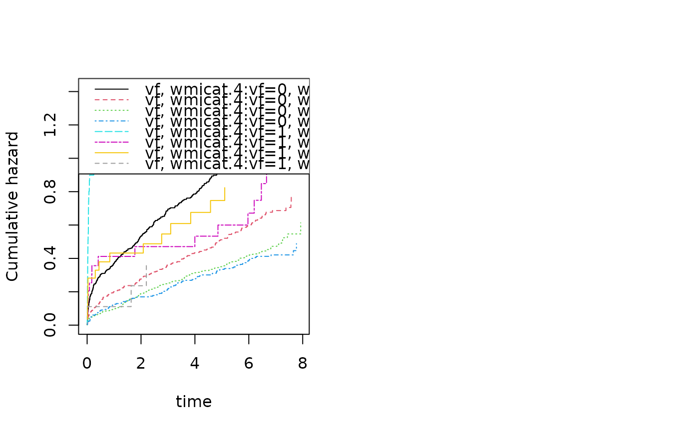
par(mfrow = c(1, 2))
plot(outs)
# IID decomposition for regression parameters
head(iid(out1))
#> wmi age
#> 3 2.315573e-04 8.113514e-05
#> 7 -1.175364e-03 -2.901628e-05
#> 13 1.826339e-03 1.670430e-04
#> 15 -3.739823e-05 2.673793e-05
#> 17 -2.997039e-03 5.371497e-05
#> 22 -9.146118e-04 -9.342247e-06
# IID decomposition for baseline at a specific time-point
Aiiid <- iid(out1, time = 30)
head(Aiiid)
#> strata0 strata1 strata2 strata3
#> 3 -1.894877e-04 -4.120570e-04 -2.659857e-04 -7.350908e-04
#> 7 1.812767e-04 2.367745e-04 1.678711e-04 8.774722e-04
#> 13 -6.837818e-04 -1.063129e-03 -6.374803e-04 -1.717426e-03
#> 15 -8.543458e-05 -9.149095e-05 -8.008394e-05 -2.250601e-04
#> 17 4.118052e-05 3.243790e-05 3.366936e-05 -1.046447e-05
#> 22 5.011669e-05 1.201129e-04 8.975026e-05 2.188617e-04
# Combined IID decomposition (beta and baseline)
dd <- iidBaseline(out1, time = 30)
head(dd$beta.iid)
#> [,1] [,2]
#> 3 2.315573e-04 8.113514e-05
#> 7 -1.175364e-03 -2.901628e-05
#> 13 1.826339e-03 1.670430e-04
#> 15 -3.739823e-05 2.673793e-05
#> 17 -2.997039e-03 5.371497e-05
#> 22 -9.146118e-04 -9.342247e-06
head(dd$base.iid)
#> strata0 strata1 strata2 strata3
#> 3 -1.894877e-04 -4.120570e-04 -2.659857e-04 -7.350908e-04
#> 7 1.812767e-04 2.367745e-04 1.678711e-04 8.774722e-04
#> 13 -6.837818e-04 -1.063129e-03 -6.374803e-04 -1.717426e-03
#> 15 -8.543458e-05 -9.149095e-05 -8.008394e-05 -2.250601e-04
#> 17 4.118052e-05 3.243790e-05 3.366936e-05 -1.046447e-05
#> 22 5.011669e-05 1.201129e-04 8.975026e-05 2.188617e-04
# Stratified model
outs <- phreg(Surv(time, status == 9) ~ strata(vf, wmicat.4) + cluster(id), data = TRACE)
summary(outs)
#>
#> n events
#> 1878 958
#>
par(mfrow = c(1, 2))
plot(outs)