Two-Stage Randomization for Competing risks and Survival outcomes
Klaus Holst & Thomas Scheike
2026-05-24
Source:vignettes/binreg-TRS.Rmd
binreg-TRS.RmdTwo-Stage Randomization for Competing risks and Survival outcomes
Under two-stage randomization we can estimate the average treatment effect E(Y(i,\bar k)) of treatment regime (i,\bar k).
- treatment A_0=i and
- for all responses, randomization A_1 = (k_1), so treatment k_1
- response\times A_1 = (k_1, k_2), so treatment k_1 if response 1, and treatment k_2 if response 2.
The estimator can be augmented in different ways: using the two randomizations and the dynamic censoring augmentation.
Estimating \mu_{i,\bar k} = P(Y(i,\bar k,\epsilon=v) <= t), restricted mean E( \min(Y(i,\bar k),\tau)) or years lost E( I(\epsilon=v) \cdot (\tau - \min(Y(i,\bar k),\tau))) using IPCW weighted estimating equations : \
The solved estimating equation is \begin{align*} \sum_i \frac{I(min(T_i,t) < G_i)}{G_c(min(T_i ,t))} I(T \leq t, \epsilon=1 ) - AUG_0 - AUG_1 + AUG_C - p(i,j)) = 0 \end{align*} using the covariates from augmentR0 to augment with \begin{align*} AUG_0 = \frac{A_0(i) - \pi_0(i)}{ \pi_0(i)} X_0 \gamma_0 \end{align*} and using the covariates from augmentR1 to augment with \begin{align*} AUG_1 = \frac{A_0(i)}{\pi_0(i)} \frac{A_1(j) - \pi_1(j)}{ \pi_1(j)} X_1 \gamma_1 \end{align*} and censoring augmenting with \begin{align*} AUG_C = \int_0^t \gamma_c(s)^T (e(s) - \bar e(s)) \frac{1}{G_c(s) } dM_c(s) \end{align*} where \gamma_c(s) is chosen to minimize the variance given the dynamic covariates specified by augmentC.
- Treatments must be given as factors.
- Treatment for the 2nd randomization may depend on response.
- Treatment probabilities are estimated by default and uncertainty from this is adjusted for.
- Randomization augmentation for the 1st and 2nd randomization is possible.
- Censoring model can be stratified on observed covariates (at time 0).
- Censoring augmentation is done dynamically over time with time-dependent covariates.
Standard errors are estimated using the influence functions of all estimators; tests of differences can therefore be computed subsequently.
Data must be in start-stop-status survival format with
- one code of
statusindicating response, i.e. 2nd randomization - other codes defining the outcome of interest
library(mets)
set.seed(100)

n <- 200
ddf <- mets:::gsim(n,covs=1,null=0,cens=1,ce=1,betac=c(0.3,1))
true <- apply(ddf$TTt<2,2,mean)
true
#> [1] 0.740 0.715 0.340 0.350
datat <- ddf$datat
## set-random response on data, only relevant after status==2
response <- rbinom(n,1,0.5)
datat$response <- as.factor(response[datat$id]*datat$Count2)
datat$A000 <- as.factor(1)
datat$A111 <- as.factor(1)

bb <- binregTSR(Event(entry,time,status)~+1+cluster(id),datat,time=2,cause=c(1),response.code=2,
        treat.model0=A0.f~+1, treat.model1=A1.f~A0.f,
        augmentR1=~X11+X12+TR, augmentR0=~X01+X02,
        augmentC=~X01+X02+A11t+A12t+X11+X12+TR, cens.model=~strata(A0.f))
bb
#> Simple estimator :
#>                              coef
#> A0.f=1, response*A1.f=1 0.5723748 0.19721139
#> A0.f=1, response*A1.f=2 0.7354573 0.08755875
#> A0.f=2, response*A1.f=1 0.2834829 0.10028201
#> A0.f=2, response*A1.f=2 0.4790373 0.10007200
#>
#> First Randomization Augmentation :
#>                              coef
#> A0.f=1, response*A1.f=1 0.5900338 0.21419118
#> A0.f=1, response*A1.f=2 0.7428143 0.08889887
#> A0.f=2, response*A1.f=1 0.2721992 0.10288280
#> A0.f=2, response*A1.f=2 0.4671886 0.10273188
#>
#> Second Randomization Augmentation :
#>                              coef
#> A0.f=1, response*A1.f=1 0.5564110 0.24533756
#> A0.f=1, response*A1.f=2 0.7185240 0.09841671
#> A0.f=2, response*A1.f=1 0.2778309 0.09021056
#> A0.f=2, response*A1.f=2 0.4685339 0.09839184
#>
#> 1st and 2nd Randomization Augmentation :
#>                              coef
#> A0.f=1, response*A1.f=1 0.5981472 0.26485855
#> A0.f=1, response*A1.f=2 0.7302633 0.10170090
#> A0.f=2, response*A1.f=1 0.2699247 0.09093482
#> A0.f=2, response*A1.f=2 0.4620365 0.09859532

estimate(coef=bb$riskG$riskG01[,1],vcov=crossprod(bb$riskG.iid$riskG01))
#>                         Estimate Std.Err    2.5%  97.5%   P-value
#> A0.f=1, response*A1.f=1   0.5981 0.26486 0.07903 1.1173 2.392e-02
#> A0.f=1, response*A1.f=2   0.7303 0.10170 0.53093 0.9296 6.946e-13
#> A0.f=2, response*A1.f=1   0.2699 0.09093 0.09170 0.4482 2.994e-03
#> A0.f=2, response*A1.f=2   0.4620 0.09860 0.26879 0.6553 2.783e-06
estimate(coef=bb$riskG$riskG01[,1],vcov=crossprod(bb$riskG.iid$riskG01),f=function(p) c(p[1]/p[2],p[3]/p[4]))
#>                         Estimate Std.Err   2.5% 97.5%  P-value
#> A0.f=1, response*A1.f=1   0.8191  0.3600 0.1135 1.525 0.022884
#> A0.f=2, response*A1.f=1   0.5842  0.2249 0.1433 1.025 0.009399
estimate(coef=bb$riskG$riskG01[,1],vcov=crossprod(bb$riskG.iid$riskG01),f=function(p) c(p[1]-p[2],p[3]-p[4]))
#>                         Estimate Std.Err    2.5%   97.5% P-value
#> A0.f=1, response*A1.f=1  -0.1321   0.266 -0.6534 0.38920  0.6194
#> A0.f=2, response*A1.f=1  -0.1921   0.129 -0.4450 0.06076  0.1365
## 2 levels for each response , fixed weights
datat$response.f <- as.factor(datat$response)
bb <- binregTSR(Event(entry,time,status)~+1+cluster(id),datat,time=2,cause=c(1),response.code=2,
        treat.model0=A0.f~+1, treat.model1=A1.f~A0.f*response.f,
        augmentR0=~X01+X02, augmentR1=~X11+X12,
        augmentC=~X01+X02+A11t+A12t+X11+X12+TR, cens.model=~strata(A0.f),
        estpr=c(0,0),pi0=0.5,pi1=0.5)
bb
#> Simple estimator :
#>                                  coef
#> A0.f=1, response.f*A1.f=1,1 0.5195752 0.18171540
#> A0.f=1, response.f*A1.f=2,1 0.5264182 0.18212146
#> A0.f=1, response.f*A1.f=1,2 0.6343225 0.09083112
#> A0.f=1, response.f*A1.f=2,2 0.6411655 0.08810024
#> A0.f=2, response.f*A1.f=1,1 0.3023142 0.11081204
#> A0.f=2, response.f*A1.f=2,1 0.3199096 0.09719853
#> A0.f=2, response.f*A1.f=1,2 0.5294417 0.13399244
#> A0.f=2, response.f*A1.f=2,2 0.5470372 0.13251846
#>
#> First Randomization Augmentation :
#>                                  coef
#> A0.f=1, response.f*A1.f=1,1 0.6359737 0.21658343
#> A0.f=1, response.f*A1.f=2,1 0.6425345 0.21728891
#> A0.f=1, response.f*A1.f=1,2 0.7129831 0.06901176
#> A0.f=1, response.f*A1.f=2,2 0.7195438 0.06513763
#> A0.f=2, response.f*A1.f=1,1 0.2561355 0.12249210
#> A0.f=2, response.f*A1.f=2,1 0.2790365 0.10488801
#> A0.f=2, response.f*A1.f=1,2 0.4557345 0.14361723
#> A0.f=2, response.f*A1.f=2,2 0.4786356 0.14226926
#>
#> Second Randomization Augmentation :
#>                                  coef
#> A0.f=1, response.f*A1.f=1,1 0.4046498 0.19742912
#> A0.f=1, response.f*A1.f=2,1 0.5687969 0.23376677
#> A0.f=1, response.f*A1.f=1,2 0.5910450 0.09523643
#> A0.f=1, response.f*A1.f=2,2 0.6498579 0.08872953
#> A0.f=2, response.f*A1.f=1,1 0.3039991 0.10638060
#> A0.f=2, response.f*A1.f=2,1 0.3311109 0.09138384
#> A0.f=2, response.f*A1.f=1,2 0.5569428 0.11332978
#> A0.f=2, response.f*A1.f=2,2 0.5164913 0.12796725
#>
#> 1st and 2nd Randomization Augmentation :
#>                                  coef
#> A0.f=1, response.f*A1.f=1,1 0.5212352 0.21098387
#> A0.f=1, response.f*A1.f=2,1 0.6994484 0.26830813
#> A0.f=1, response.f*A1.f=1,2 0.6692919 0.07617047
#> A0.f=1, response.f*A1.f=2,2 0.7328127 0.06615399
#> A0.f=2, response.f*A1.f=1,1 0.2586853 0.11531506
#> A0.f=2, response.f*A1.f=2,1 0.2935352 0.09702298
#> A0.f=2, response.f*A1.f=1,2 0.4809089 0.11457277
#> A0.f=2, response.f*A1.f=2,2 0.4602799 0.13349781

## 2 levels for each response ,  estimated treat probabilities
bb <- binregTSR(Event(entry,time,status)~+1+cluster(id),datat,time=2,cause=c(1),response.code=2,
        treat.model0=A0.f~+1, treat.model1=A1.f~A0.f*response.f,
        augmentR0=~X01+X02, augmentR1=~X11+X12,
        augmentC=~X01+X02+A11t+A12t+X11+X12+TR, cens.model=~strata(A0.f),estpr=c(1,1))
bb
#> Simple estimator :
#>                                  coef
#> A0.f=1, response.f*A1.f=1,1 0.5733301 0.25088070
#> A0.f=1, response.f*A1.f=2,1 0.6022300 0.25101611
#> A0.f=1, response.f*A1.f=1,2 0.6893786 0.07700325
#> A0.f=1, response.f*A1.f=2,2 0.7182785 0.08178121
#> A0.f=2, response.f*A1.f=1,1 0.2851197 0.09997901
#> A0.f=2, response.f*A1.f=2,1 0.2841367 0.07893846
#> A0.f=2, response.f*A1.f=1,2 0.4821020 0.10343782
#> A0.f=2, response.f*A1.f=2,2 0.4811190 0.10002228
#>
#> First Randomization Augmentation :
#>                                  coef
#> A0.f=1, response.f*A1.f=1,1 0.5934059 0.27131225
#> A0.f=1, response.f*A1.f=2,1 0.6224367 0.27204244
#> A0.f=1, response.f*A1.f=1,2 0.6962560 0.07772829
#> A0.f=1, response.f*A1.f=2,2 0.7252868 0.08319005
#> A0.f=2, response.f*A1.f=1,1 0.2738115 0.10244557
#> A0.f=2, response.f*A1.f=2,1 0.2767634 0.08081569
#> A0.f=2, response.f*A1.f=1,2 0.4661741 0.10481333
#> A0.f=2, response.f*A1.f=2,2 0.4691260 0.10238718
#>
#> Second Randomization Augmentation :
#>                                  coef
#> A0.f=1, response.f*A1.f=1,1 0.4372672 0.23706174
#> A0.f=1, response.f*A1.f=2,1 0.5854429 0.26329507
#> A0.f=1, response.f*A1.f=1,2 0.6685369 0.07730893
#> A0.f=1, response.f*A1.f=2,2 0.7320359 0.08145477
#> A0.f=2, response.f*A1.f=1,1 0.2745442 0.10426421
#> A0.f=2, response.f*A1.f=2,1 0.2988823 0.07578047
#> A0.f=2, response.f*A1.f=1,2 0.5019477 0.09984288
#> A0.f=2, response.f*A1.f=2,2 0.4745778 0.10218550
#>
#> 1st and 2nd Randomization Augmentation :
#>                                  coef
#> A0.f=1, response.f*A1.f=1,1 0.4702327 0.25293879
#> A0.f=1, response.f*A1.f=2,1 0.6127080 0.28587900
#> A0.f=1, response.f*A1.f=1,2 0.6759149 0.07701506
#> A0.f=1, response.f*A1.f=2,2 0.7433289 0.08370622
#> A0.f=2, response.f*A1.f=1,1 0.2634297 0.10565890
#> A0.f=2, response.f*A1.f=2,1 0.2948997 0.07656016
#> A0.f=2, response.f*A1.f=1,2 0.4865367 0.09860797
#> A0.f=2, response.f*A1.f=2,2 0.4699980 0.10193373


## 2 and 3 levels for each response , fixed weights
datat$A1.23.f <- as.numeric(datat$A1.f)
dtable(datat,~A1.23.f+response)
#>
#>         response   0   1
#> A1.23.f
#> 1                120  23
#> 2                120  25
datat <- dtransform(datat,A1.23.f=2+rbinom(nrow(datat),1,0.5),
            Count2==1 & A1.23.f==2 & response==0)
dtable(datat,~A1.23.f+response)
#>
#>         response   0   1
#> A1.23.f
#> 1                120  23
#> 2                111  25
#> 3                  9   0
datat$A1.23.f <- as.factor(datat$A1.23.f)
dtable(datat,~A1.23.f+response|Count2==1)
#>
#>         response  0  1
#> A1.23.f
#> 1                21 23
#> 2                10 25
#> 3                 9  0
###
bb <- binregTSR(Event(entry,time,status)~+1+cluster(id),datat,time=2,cause=c(1),response.code=2,
    treat.model0=A0.f~+1,treat.model1=A1.23.f~A0.f*response.f,
    augmentR0=~X01+X02, augmentR1=~X11+X12,
    augmentC=~X01+X02+A11t+A12t+X11+X12+TR, cens.model=~strata(A0.f),
        estpr=c(1,0),pi1=c(0.3,0.5))
bb
#> Simple estimator :
#>                                     coef
#> A0.f=1, response.f*A1.23.f=1,1 0.5928568 0.20464868
#> A0.f=1, response.f*A1.23.f=2,1 0.6055291 0.20241441
#> A0.f=1, response.f*A1.23.f=3,1 0.5539792 0.19865003
#> A0.f=1, response.f*A1.23.f=1,2 0.7203538 0.09728960
#> A0.f=1, response.f*A1.23.f=2,2 0.7330260 0.08618558
#> A0.f=1, response.f*A1.23.f=3,2 0.6814762 0.07905734
#> A0.f=2, response.f*A1.23.f=1,1 0.3487105 0.14756981
#> A0.f=2, response.f*A1.23.f=2,1 0.2724117 0.09182351
#> A0.f=2, response.f*A1.23.f=3,1 0.2669705 0.10319223
#> A0.f=2, response.f*A1.23.f=1,2 0.5551901 0.15399346
#> A0.f=2, response.f*A1.23.f=2,2 0.4788913 0.12263546
#> A0.f=2, response.f*A1.23.f=3,2 0.4734501 0.12853150
#>
#> First Randomization Augmentation :
#>                                     coef
#> A0.f=1, response.f*A1.23.f=1,1 0.6091794 0.22507560
#> A0.f=1, response.f*A1.23.f=2,1 0.6246762 0.22364858
#> A0.f=1, response.f*A1.23.f=3,1 0.5756603 0.21982886
#> A0.f=1, response.f*A1.23.f=1,2 0.7242102 0.10066515
#> A0.f=1, response.f*A1.23.f=2,2 0.7397070 0.08813234
#> A0.f=1, response.f*A1.23.f=3,2 0.6906911 0.07986256
#> A0.f=2, response.f*A1.23.f=1,1 0.3348012 0.15239160
#> A0.f=2, response.f*A1.23.f=2,1 0.2718558 0.09060009
#> A0.f=2, response.f*A1.23.f=3,1 0.2532931 0.10673462
#> A0.f=2, response.f*A1.23.f=1,2 0.5362379 0.15754640
#> A0.f=2, response.f*A1.23.f=2,2 0.4732925 0.12378699
#> A0.f=2, response.f*A1.23.f=3,2 0.4547298 0.13192021
#>
#> Second Randomization Augmentation :
#>                                     coef
#> A0.f=1, response.f*A1.23.f=1,1 0.4707095 0.21804098
#> A0.f=1, response.f*A1.23.f=2,1 0.6287053 0.22907037
#> A0.f=1, response.f*A1.23.f=3,1 0.6778953 0.30311581
#> A0.f=1, response.f*A1.23.f=1,2 0.6499002 0.12488660
#> A0.f=1, response.f*A1.23.f=2,2 0.7656237 0.07140976
#> A0.f=1, response.f*A1.23.f=3,2 0.6875010 0.08312068
#> A0.f=2, response.f*A1.23.f=1,1 0.2656521 0.17396985
#> A0.f=2, response.f*A1.23.f=2,1 0.2706333 0.08715854
#> A0.f=2, response.f*A1.23.f=3,1 0.3235400 0.07994612
#> A0.f=2, response.f*A1.23.f=1,2 0.4759907 0.16071698
#> A0.f=2, response.f*A1.23.f=2,2 0.4671860 0.11714753
#> A0.f=2, response.f*A1.23.f=3,2 0.5050170 0.11067832
#>
#> 1st and 2nd Randomization Augmentation :
#>                                     coef
#> A0.f=1, response.f*A1.23.f=1,1 0.5068915 0.22640669
#> A0.f=1, response.f*A1.23.f=2,1 0.6601925 0.25328437
#> A0.f=1, response.f*A1.23.f=3,1 0.7128045 0.32561624
#> A0.f=1, response.f*A1.23.f=1,2 0.6681178 0.12092323
#> A0.f=1, response.f*A1.23.f=2,2 0.7709766 0.07310528
#> A0.f=1, response.f*A1.23.f=3,2 0.7088981 0.08171051
#> A0.f=2, response.f*A1.23.f=1,1 0.2472033 0.17493179
#> A0.f=2, response.f*A1.23.f=2,1 0.2703258 0.08650158
#> A0.f=2, response.f*A1.23.f=3,1 0.3183141 0.08043082
#> A0.f=2, response.f*A1.23.f=1,2 0.4540746 0.15704473
#> A0.f=2, response.f*A1.23.f=2,2 0.4667557 0.11617870
#> A0.f=2, response.f*A1.23.f=3,2 0.4960792 0.11127903


## 2 and 3 levels for each response , estimated
bb <- binregTSR(Event(entry,time,status)~+1+cluster(id),datat,time=2,cause=c(1),response.code=2,
    treat.model0=A0.f~+1, treat.model1=A1.23.f~A0.f*response.f,
    augmentR0=~X01+X02, augmentR1=~X11+X12,
    augmentC=~X01+X02+A11t+A12t+X11+X12+TR,cens.model=~strata(A0.f),
    estpr=c(1,1))
bb
#> Simple estimator :
#>                                     coef
#> A0.f=1, response.f*A1.23.f=1,1 0.5733301 0.25088123
#> A0.f=1, response.f*A1.23.f=2,1 0.6486249 0.25863637
#> A0.f=1, response.f*A1.23.f=3,1 0.5558352 0.25058134
#> A0.f=1, response.f*A1.23.f=1,2 0.6893788 0.07700333
#> A0.f=1, response.f*A1.23.f=2,2 0.7646736 0.11893993
#> A0.f=1, response.f*A1.23.f=3,2 0.6718839 0.07549715
#> A0.f=2, response.f*A1.23.f=1,1 0.2851198 0.09997906
#> A0.f=2, response.f*A1.23.f=2,1 0.2795959 0.10086233
#> A0.f=2, response.f*A1.23.f=3,1 0.2893264 0.12751179
#> A0.f=2, response.f*A1.23.f=1,2 0.4821024 0.10343788
#> A0.f=2, response.f*A1.23.f=2,2 0.4765785 0.12129977
#> A0.f=2, response.f*A1.23.f=3,2 0.4863090 0.13928327
#>
#> First Randomization Augmentation :
#>                                     coef
#> A0.f=1, response.f*A1.23.f=1,1 0.5934060 0.27131280
#> A0.f=1, response.f*A1.23.f=2,1 0.6665511 0.27965619
#> A0.f=1, response.f*A1.23.f=3,1 0.5783224 0.27132992
#> A0.f=1, response.f*A1.23.f=1,2 0.6962562 0.07772837
#> A0.f=1, response.f*A1.23.f=2,2 0.7694013 0.12078013
#> A0.f=1, response.f*A1.23.f=3,2 0.6811727 0.07593118
#> A0.f=2, response.f*A1.23.f=1,1 0.2738116 0.10244561
#> A0.f=2, response.f*A1.23.f=2,1 0.2791785 0.10064910
#> A0.f=2, response.f*A1.23.f=3,1 0.2740035 0.13235513
#> A0.f=2, response.f*A1.23.f=1,2 0.4661745 0.10481340
#> A0.f=2, response.f*A1.23.f=2,2 0.4715413 0.12263585
#> A0.f=2, response.f*A1.23.f=3,2 0.4663664 0.14396909
#>
#> Second Randomization Augmentation :
#>                                     coef
#> A0.f=1, response.f*A1.23.f=1,1 0.4372664 0.23706211
#> A0.f=1, response.f*A1.23.f=2,1 0.5867572 0.24940274
#> A0.f=1, response.f*A1.23.f=3,1 0.6818858 0.34853309
#> A0.f=1, response.f*A1.23.f=1,2 0.6685368 0.07730905
#> A0.f=1, response.f*A1.23.f=2,2 0.7678408 0.07768404
#> A0.f=1, response.f*A1.23.f=3,2 0.6794316 0.07967452
#> A0.f=2, response.f*A1.23.f=1,1 0.2745441 0.10426433
#> A0.f=2, response.f*A1.23.f=2,1 0.2695053 0.09394894
#> A0.f=2, response.f*A1.23.f=3,1 0.3345432 0.09931154
#> A0.f=2, response.f*A1.23.f=1,2 0.5019478 0.09984303
#> A0.f=2, response.f*A1.23.f=2,2 0.4603587 0.11962056
#> A0.f=2, response.f*A1.23.f=3,2 0.5047271 0.12508846
#>
#> 1st and 2nd Randomization Augmentation :
#>                                     coef
#> A0.f=1, response.f*A1.23.f=1,1 0.4702319 0.25293915
#> A0.f=1, response.f*A1.23.f=2,1 0.6117617 0.26980849
#> A0.f=1, response.f*A1.23.f=3,1 0.7132649 0.36786766
#> A0.f=1, response.f*A1.23.f=1,2 0.6759149 0.07701519
#> A0.f=1, response.f*A1.23.f=2,2 0.7733904 0.07957475
#> A0.f=1, response.f*A1.23.f=3,2 0.7066309 0.07677686
#> A0.f=2, response.f*A1.23.f=1,1 0.2634296 0.10565903
#> A0.f=2, response.f*A1.23.f=2,1 0.2691166 0.09330578
#> A0.f=2, response.f*A1.23.f=3,1 0.3296791 0.10056744
#> A0.f=2, response.f*A1.23.f=1,2 0.4865368 0.09860813
#> A0.f=2, response.f*A1.23.f=2,2 0.4605674 0.11777635
#> A0.f=2, response.f*A1.23.f=3,2 0.4971161 0.12478451


## 2 and 1 level for each response
datat$A1.21.f <- as.numeric(datat$A1.f)
dtable(datat,~A1.21.f+response|Count2==1)
#>
#>         response  0  1
#> A1.21.f
#> 1                21 23
#> 2                19 25
datat <- dtransform(datat,A1.21.f=1,Count2==1 & response==1)
dtable(datat,~A1.21.f+response|Count2==1)
#>
#>         response  0  1
#> A1.21.f
#> 1                21 48
#> 2                19  0
datat$A1.21.f <- as.factor(datat$A1.21.f)
dtable(datat,~A1.21.f+response|Count2==1)
#>
#>         response  0  1
#> A1.21.f
#> 1                21 48
#> 2                19  0
bb <- binregTSR(Event(entry,time,status)~+1+cluster(id),datat,time=2,cause=c(1),response.code=2,
    treat.model0=A0.f~+1, treat.model1=A1.21.f~A0.f*response.f,
    augmentR0=~X01+X02, augmentR1=~X11+X12,
    augmentC=~X01+X02+A11t+A12t+X11+X12+TR,cens.model=~strata(A0.f),
    estpr=c(1,1))
bb
#> Simple estimator :
#>                                     coef
#> A0.f=1, response.f*A1.21.f=1,1 0.6352226 0.11813045
#> A0.f=1, response.f*A1.21.f=2,1 0.6641226 0.12002926
#> A0.f=2, response.f*A1.21.f=1,1 0.3865954 0.09118205
#> A0.f=2, response.f*A1.21.f=2,1 0.3856124 0.07700508
#>
#> First Randomization Augmentation :
#>                                     coef
#> A0.f=1, response.f*A1.21.f=1,1 0.6482593 0.12794220
#> A0.f=1, response.f*A1.21.f=2,1 0.6772901 0.13063539
#> A0.f=2, response.f*A1.21.f=1,1 0.3729074 0.09195877
#> A0.f=2, response.f*A1.21.f=2,1 0.3758593 0.07808807
#>
#> Second Randomization Augmentation :
#>                                     coef
#> A0.f=1, response.f*A1.21.f=1,1 0.6435175 0.11802262
#> A0.f=1, response.f*A1.21.f=2,1 0.6882148 0.11332360
#> A0.f=2, response.f*A1.21.f=1,1 0.3954927 0.09148962
#> A0.f=2, response.f*A1.21.f=2,1 0.3782504 0.08450470
#>
#> 1st and 2nd Randomization Augmentation :
#>                                     coef
#> A0.f=1, response.f*A1.21.f=1,1 0.6685224 0.13033444
#> A0.f=1, response.f*A1.21.f=2,1 0.7138566 0.12655030
#> A0.f=2, response.f*A1.21.f=1,1 0.3839378 0.08986106
#> A0.f=2, response.f*A1.21.f=2,1 0.3758166 0.08434474

## known weights
bb <- binregTSR(Event(entry,time,status)~+1+cluster(id),datat,time=2,cause=c(1),response.code=2,
    treat.model0=A0.f~+1, treat.model1=A1.21.f~A0.f*response.f,
    augmentR0=~X01+X02, augmentR1=~X11+X12,
    augmentC=~X01+X02+A11t+A12t+X11+X12+TR,
    cens.model=~strata(A0.f),estpr=c(1,0),pi1=c(0.5,1))
bb
#> Simple estimator :
#>                                     coef
#> A0.f=1, response.f*A1.21.f=1,1 0.6410543 0.12005600
#> A0.f=1, response.f*A1.21.f=2,1 0.6486576 0.11864403
#> A0.f=2, response.f*A1.21.f=1,1 0.3780709 0.09171015
#> A0.f=2, response.f*A1.21.f=2,1 0.3940667 0.08377301
#>
#> First Randomization Augmentation :
#>                                     coef
#> A0.f=1, response.f*A1.21.f=1,1 0.6532872 0.12997608
#> A0.f=1, response.f*A1.21.f=2,1 0.6625853 0.12899925
#> A0.f=2, response.f*A1.21.f=1,1 0.3647406 0.09331039
#> A0.f=2, response.f*A1.21.f=2,1 0.3842369 0.08422015
#>
#> Second Randomization Augmentation :
#>                                     coef
#> A0.f=1, response.f*A1.21.f=1,1 0.6435110 0.12122751
#> A0.f=1, response.f*A1.21.f=2,1 0.6751763 0.11432293
#> A0.f=2, response.f*A1.21.f=1,1 0.3957743 0.08413935
#> A0.f=2, response.f*A1.21.f=2,1 0.3772145 0.09110553
#>
#> 1st and 2nd Randomization Augmentation :
#>                                     coef
#> A0.f=1, response.f*A1.21.f=1,1 0.6709750 0.13165583
#> A0.f=1, response.f*A1.21.f=2,1 0.7043078 0.12732297
#> A0.f=2, response.f*A1.21.f=1,1 0.3861201 0.08279377
#> A0.f=2, response.f*A1.21.f=2,1 0.3757694 0.09080739
Two-Stage Randomization CALGB-9823
We illustrate an analysis of one SMART conducted by Cancer and Leukemia Group B Protocol 8923 (CALGB 8923), Stone et al. (2001). 388 patients were randomized to an initial treatment of GM-CSF (A_1) or standard chemotherapy (A_2). Patients with complete remission and informed consent to the second stage were then re-randomized to cytarabine only (B_1) or cytarabine plus mitoxantrone (B_2).
We first compute the weighted risk-set estimator based on estimated weights \begin{align*} \Lambda_{A1,B1}(t) & = \sum_i \int_0^t \frac{w_i(s)}{Y^w(s)} dN_i(s) \end{align*} where w_i(s) = I(A0_i=A1) + I(t>T_R) I(A1_i=B1)/\pi_1(X_i), that is 1 when starting on treatment A1, and then scaled up by the proportion switching to B1 at time T_R for those that do so. This is equivalent to the IPTW (inverse probability of treatment weighted) estimator. We estimate the treatment regimes A1, B1 and A2, B1 by letting A10 indicate those consistent with ending on B1. A10 starts at 1 and becomes 0 if the subject is treated with B2, but stays 1 if treated with B1. We can then look at the two strata where A0=0, A10=1 and A0=1, A10=1. Similarly, we define A11 to start at 1, remain 1 if B2 is taken, and become 0 if the second randomization is B1.
- the treatment models apply to all time-points, unless the
weight.varvariable is given (1 for treatments, 0 otherwise) to accommodate a general start-stop format - the treatment model may also depend on a response value
- standard errors are based on influence functions and are also computed for the baseline
We here use the propensity score model P(A1=B1|A0) that uses the observed frequencies on arm B1 among those starting out on either A1 or A2.
data(calgb8923)
calgt <- calgb8923

tm=At.f~factor(Count2)+age+sex+wbc
tm=At.f~factor(Count2)
tm=At.f~factor(Count2)*A0.f

head(calgt)
#>   id V X Z   TR R     U delta  stop age   wbc sex race      time status start
#> 1  1 0 0 0 0.00 0 13.33     1 13.33  64 128.0   1    1 13.338219      1  0.00
#> 2  2 1 1 0 0.00 0 17.80     1 17.80  71   4.3   2    1 17.802995      1  0.00
#> 3  3 1 0 0 0.00 0  1.27     1  1.27  71  43.6   2    1  1.271527      1  0.00
#> 4  4 1 0 1 0.00 0 24.77     1 24.77  63  72.3   2    1  0.730000      2  0.00
#> 5  4 1 0 1 0.73 1 24.77     1 24.77  63  72.3   2    1 24.772515      1  0.73
#> 6  5 0 1 0 0.00 0 10.37     1 10.37  65   1.4   1    1 10.374479      1  0.00
#>   A0.f A0 A1 A11 A12 A1.f A10 At.f lbnr__id Count1 Count2 consent trt2 trt1
#> 1    0  0  0   1   0    0   0    0        1      0      0      -1   -1    1
#> 2    1  1  0   1   0    0   0    1        1      0      0      -1   -1    2
#> 3    0  0  0   1   0    0   0    0        1      0      0      -1   -1    1
#> 4    0  0  0   1   0    0   0    0        1      0      0      -1   -1    1
#> 5    0  0  1   1   1    1   1    1        2      0      1       1    1    1
#> 6    1  1  0   1   0    0   0    1        1      0      0      -1   -1    2
ll0 <- phreg_IPTW(Event(start,time,status==1)~strata(A0,A10)+cluster(id),calgt,treat.model=tm)
pll0 <- predict(ll0,expand.grid(A0=0:1,A10=0,id=1))
ll1 <- phreg_IPTW(Event(start,time,status==1)~strata(A0,A11)+cluster(id),calgt,treat.model=tm)
pll1 <- predict(ll1,expand.grid(A0=0:1,A11=1,id=1))
plot(pll0,se=1,lwd=2,col=1:2,lty=1,xlab="time (months)",xlim=c(0,30))
plot(pll1,add=TRUE,col=3:4,se=1,lwd=2,lty=1,xlim=c(0,30))
abline(h=0.25)
legend("topright",c("A1B1","A2B1","A1B2","A2B2"),col=c(1,2,3,4),lty=1)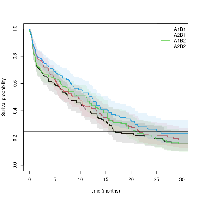
summary(pll1,times=12)
#> Predictions of type 'surv'
#>   Showing subjects: 1, 2
#>   Showing times:    12
#>
#> -- Subject 1 --
#>  time   surv     se  lower  upper
#>    12 0.4557 0.0421 0.3801 0.5462
#>
#> -- Subject 2 --
#>  time   surv     se  lower  upper
#>    12 0.5029 0.0417 0.4276 0.5916
summary(pll0,times=12)
#> Predictions of type 'surv'
#>   Showing subjects: 1, 2
#>   Showing times:    12
#>
#> -- Subject 1 --
#>  time  surv     se  lower  upper
#>    12 0.395 0.0426 0.3197 0.4881
#>
#> -- Subject 2 --
#>  time   surv     se  lower  upper
#>    12 0.4279 0.0434 0.3507 0.5221
The propensity score model can be extended to use covariates to get increased efficiency. Note also that the propensity scores for A0 will cancel out in the different strata.
SessionInfo
sessionInfo()
#> R version 4.6.0 (2026-04-24)
#> Platform: x86_64-pc-linux-gnu
#> Running under: Ubuntu 24.04.4 LTS
#>
#> Matrix products: default
#> BLAS:   /home/kkzh/.asdf/installs/r/4.6.0/lib/R/lib/libRblas.so
#> LAPACK: /usr/lib/x86_64-linux-gnu/lapack/liblapack.so.3.12.0  LAPACK version 3.12.0
#>
#> locale:
#>  [1] LC_CTYPE=en_US.UTF-8       LC_NUMERIC=C
#>  [3] LC_TIME=en_US.UTF-8        LC_COLLATE=en_US.UTF-8
#>  [5] LC_MONETARY=en_US.UTF-8    LC_MESSAGES=en_US.UTF-8
#>  [7] LC_PAPER=en_US.UTF-8       LC_NAME=C
#>  [9] LC_ADDRESS=C               LC_TELEPHONE=C
#> [11] LC_MEASUREMENT=en_US.UTF-8 LC_IDENTIFICATION=C
#>
#> time zone: Europe/Copenhagen
#> tzcode source: system (glibc)
#>
#> attached base packages:
#> [1] stats     graphics  grDevices utils     datasets  methods   base
#>
#> other attached packages:
#> [1] timereg_2.0.7  survival_3.8-6 mets_1.3.10
#>
#> loaded via a namespace (and not attached):
#>  [1] cli_3.6.6              knitr_1.51             rlang_1.2.0
#>  [4] xfun_0.57              otel_0.2.0             future.apply_1.20.2
#>  [7] listenv_0.10.1         lava_1.9.1             stats4_4.6.0
#> [10] grid_4.6.0             evaluate_1.0.5         yaml_2.3.12
#> [13] mvtnorm_1.3-7          numDeriv_2016.8-1.1    compiler_4.6.0
#> [16] codetools_0.2-20       Rcpp_1.1.1-1.1         ucminf_1.2.3
#> [19] future_1.70.0          lattice_0.22-9         digest_0.6.39
#> [22] parallelly_1.47.0      parallel_4.6.0         splines_4.6.0
#> [25] Matrix_1.7-5           tools_4.6.0            RcppArmadillo_15.2.6-1
#> [28] globals_0.19.1