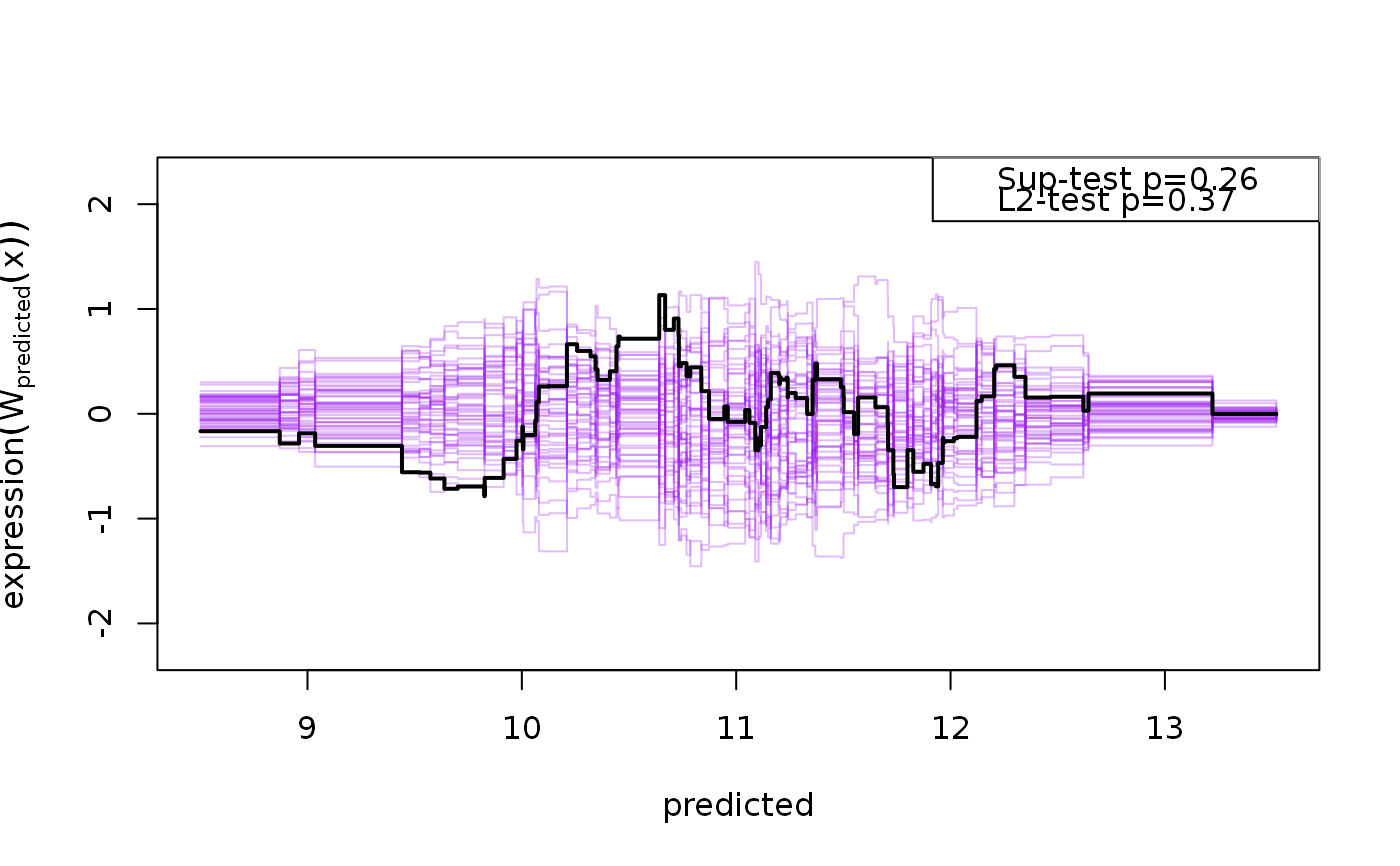
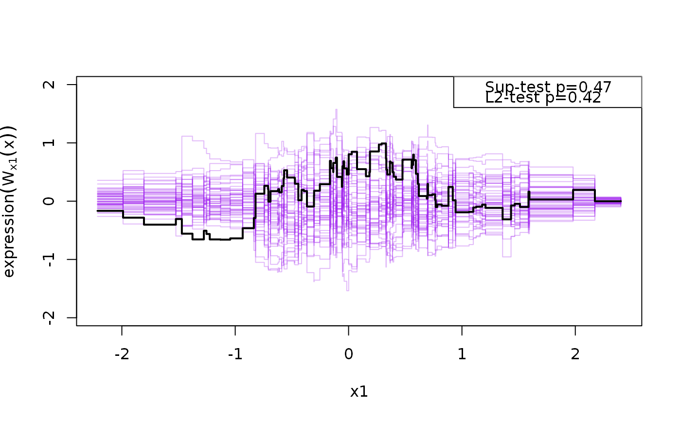
Calculates GoF statistics based on cumulative residual processes

Given the generalized linear models model $$g(E(Y_i|X_{i1},...,X_{ik})) = \sum_{i=1}^k \beta_jX_{ij}$$ the cumres-function calculates the the observed cumulative sum of residual process, cumulating the residuals, $e_i$, by the jth covariate: $$W_j(t) = n^{-1/2}\sum_{i=1}^n 1_{\{X_{ij}<t\}}e_i$$ and Sup and L2 test statistics are calculated via simulation from the asymptotic distribution of the cumulative residual process under the null (Lin et al., 2002).

# S3 method for glm
cumres(
  model,
  variable = c("predicted", colnames(model.matrix(model))),
  data = data.frame(model.matrix(model)),
  R = 1000,
  b = 0,
  plots = min(R, 50),
  ...
)

Arguments

model	Model object (`lm` or `glm`)
variable	List of variable to order the residuals after
data	data.frame used to fit model (complete cases)
R	Number of samples used in simulation
b	Moving average bandwidth (0 corresponds to infinity = standard cumulated residuals)
plots	Number of realizations to save for use in the plot-routine
...	additional arguments

Value

Returns an object of class 'cumres'.

Note

Currently linear (normal), logistic and poisson regression models with canonical links are supported.

References

D.Y. Lin and L.J. Wei and Z. Ying (2002) Model-Checking Techniques Based on Cumulative Residuals. Biometrics, Volume 58, pp 1-12.

John Q. Su and L.J. Wei (1991) A lack-of-fit test for the mean function in a generalized linear model. Journal. Amer. Statist. Assoc., Volume 86, Number 414, pp 420-426.

Author

Klaus K. Holst

Examples


sim1 <- function(n=100, f=function(x1,x2) {10+x1+x2^2}, sd=1, seed=1) {
  if (!is.null(seed))
    set.seed(seed)
  x1 <- rnorm(n);
  x2 <- rnorm(n)
  X <- cbind(1,x1,x2)
  y <- f(x1,x2) + rnorm(n,sd=sd)
  d <- data.frame(y,x1,x2)
  return(d)
}
d <- sim1(100); l <- lm(y ~ x1 + x2,d)
system.time(g <- cumres(l, R=100, plots=50))
#>    user  system elapsed 
#>   0.023   0.001   0.023 
g
#> 
#>           p-value(Sup) p-value(L2)
#> predicted         0.26        0.37
#> x1                0.47        0.42
#> x2                0.00        0.00
#> 
#> Based on 100 realizations.
plot(g)
g1 <- cumres(l, c("y"), R=100, plots=50)
g1
#> 
#>           p-value(Sup) p-value(L2)
#> predicted         0.35        0.35
#> 
#> Based on 100 realizations.
g2 <- cumres(l, c("y"), R=100, plots=50, b=0.5)
g2
#> 
#>           p-value(Sup) p-value(L2)
#> predicted         0.21        0.26
#> 
#> Based on 100 realizations.